Budgeted Cost-Aware Policy Comparison

Overview

This example checks whether the cost-aware active-learning policy responds sensibly to the relative cost of function and derivative observations. The idea is to compare the policy against deliberately restricted baselines under the same budget:

• when derivatives are cheap, compare against a function-only policy,

• when function values are cheap, compare against a derivative-only policy.

All runs use the same Branin-Hoo function, initial design, GP fitting code, test grid, optimizer settings, and budget accounting. The only difference is which candidate types each policy is allowed to select.

—

Baseline Policies

The baselines are intentionally simple. They subclass AdaptiveDirectionalGP and filter the candidate set before the best candidate is chosen.

class CandidateFilteredAdaptiveGP(AdaptiveDirectionalGP):
    allowed_kind = None

    def _build_cost_aware_candidates(self):
        candidates = super()._build_cost_aware_candidates()
        if self.allowed_kind is None:
            return candidates
        return [c for c in candidates if c.kind == self.allowed_kind]

class FunctionOnlyAdaptiveGP(CandidateFilteredAdaptiveGP):
    allowed_kind = "f"

class DerivativeOnlyAdaptiveGP(CandidateFilteredAdaptiveGP):
    allowed_kind = "d"

This is useful because the baselines still use the same GP implementation and cost-budget logic as the cost-aware policy. The comparison isolates the candidate-selection decision rather than comparing against a separate code path.

—

Experiment 1: Derivatives Are Cheap

In the first regime, a function value costs ten times as much as a first-order directional derivative:

• c_f = 10

• c1 = 1

• budget B = 20

The function-only baseline can afford only two new function evaluations. The cost-aware policy can instead spend the same budget on multiple derivative observations at existing sites (with at most one additional function evaluation if its uncertainty-per-cost score wins).

—

Experiment 2: Function Values Are Cheap

In the second regime, the cost relationship is reversed:

• c_f = 1

• c1 = 10

• budget B = 20

The derivative-only baseline can afford only two derivative observations. The cost-aware policy should instead spend most of the budget on additional function evaluations.

—

Results

The figure shows grid RMSE for each policy in the two cost regimes. The text above each bar gives the selected observation sequence: f for a function evaluation and d for a derivative observation.

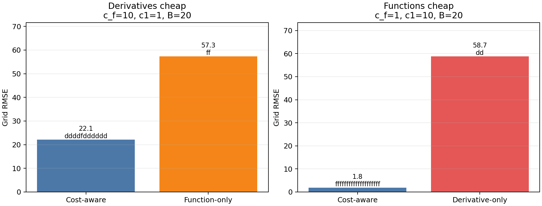
The generated run produced the following table:

Cost-aware policy comparison

Regime	Policy	Selected observations	Cost used	Grid RMSE
Derivatives cheap (c_f=10, c1=1, B=20)	Cost-aware	ddddfdddddd	20.0	22.10
Derivatives cheap (c_f=10, c1=1, B=20)	Function-only	ff	20.0	57.26
Functions cheap (c_f=1, c1=10, B=20)	Cost-aware	ffffffffffffffffffff	20.0	1.80
Functions cheap (c_f=1, c1=10, B=20)	Derivative-only	dd	20.0	58.74

Interpretation

The cost-aware policy changes behavior when the cost model changes:

• when derivatives are cheap, it selects derivative observations and beats the function-only budget baseline;

• when derivatives are too expensive, it selects function observations and beats the derivative-only baseline.

This is not intended to prove global optimality. It is a regression-style sanity check that the implementation uses the cost model in a useful way.

Reproducing the Figure

Run:

python docs/source/JetGP_module_examples/active_learning/active_learning_cost_comparison.py

The script writes:

• docs/source/_static/active_learning_cost_comparison.png

The same comparison is also covered by the active-learning test suite in active_learning/tests/test_cost_aware_value.py.