JetGP#
A Gaussian Process library with support for arbitrary-order derivative-enhanced training data.
Module Overview#
JetGP provides four main modules for derivative-enhanced Gaussian Process modeling:
Core Modules
DEGP (Derivative-Enhanced GP): Uses coordinate-aligned partial derivatives (∂f/∂x₁, ∂f/∂x₂, etc.). Best for problems where axis-aligned sensitivities are natural.
DDEGP (Directional Derivative-Enhanced GP): Uses global directional derivatives with fixed ray directions applied at all (or a subset of) training points. Efficient when derivative information is available along consistent directions across the domain.
GDDEGP (Generalized Directional Derivative-Enhanced GP): Uses point-wise directional derivatives where each training point can have unique ray directions. Ideal for adaptive methods where derivative directions vary spatially (e.g., gradient-aligned sampling).
Unified Submodeling Framework
WDEGP (Weighted Derivative-Enhanced GP): A unified framework for combining multiple submodels, each trained on different subsets of training points with different derivative configurations. Supports submodeling with any of the core module types via the
submodel_typeparameter ('degp','ddegp', or'gddegp').
Module |
Derivative Type |
Ray Specification |
Use Case |
|---|---|---|---|
DEGP |
Partial derivatives |
N/A (coordinate-aligned) |
Standard derivative data |
DDEGP |
Directional derivatives |
Global |
Fixed directions across domain |
GDDEGP |
Directional derivatives |
Point-wise |
Spatially-varying directions |
WDEGP |
Any of the above |
Depends on |
Partitioned training data |
Installation#
Anaconda#
Ensure that the Anaconda distribution is installed on your system. Click here for installation steps.
Cloning the repository#
$ git clone git@github.com:Samm-Py/jetgp.git
Conda environment#
Set up the dependencies of this repository using the environment.yml file.
Go to the root of the cloned repository. Create and activate the conda environment with the supplied
environment.ymlfile at root:
$ cd <path-to-JetGP>
$ conda env create -f environment.yml
$ conda activate jetgp
In the event where dependencies are added, the jetgp environment can be updated:
$ conda env update --file environment.yml --prune
Add JetGP to Python Path#
To make the jetgp library importable from anywhere, it must be added to your Python path.
There are two recommended ways to do this:
Option 1: Temporary addition using ``PYTHONPATH``
# From  ``.\jetgp-main``
$ export PYTHONPATH=$PYTHONPATH:$(pwd)

# Optional: verify that JetGP is accessible
$ python -c "import jetgp; print('JetGP successfully added to PYTHONPATH')"
To make this change permanent, add the export line to your shell configuration file (e.g., ~/.bashrc or ~/.zshrc).
Option 2: Persistent addition using Conda (recommended for Anaconda users)
If using Anaconda, you can register the repository path with your environment using conda develop
$ cd <path-to-JetGP> (e.g., ``.\jetgp-main``).
$ conda develop .
This method automatically makes jetgp importable whenever the jetgp environment is active.
Local documentation build#
The documentation of the library can be built locally.
Ensure that the conda environment is activated:
$ conda activate jetgp
Change directory to the
docsdirectory and make abuilddirectory:
$ cd docs
$ mkdir build
Build and open the HTML documentation (e.g., using Firefox browser):
$ sphinx-build -M html source build
$ cd build/html
$ firefox index.html
Quick Start Examples#
DEGP: Derivative-Enhanced Gaussian Process#
DEGP uses coordinate-aligned partial derivatives (∂f/∂x₁, ∂²f/∂x₁², etc.) for training.
This example demonstrates DEGP on the 2D function \(f(x_1, x_2) = \sin(x_1)\cos(x_2)\) using a 3×3 training grid with first and second-order coordinate derivatives.
import numpy as np
from jetgp.full_degp.degp import degp
import matplotlib.pyplot as plt

# Generate 3x3 training grid
X1 = np.array([0.0, 0.5, 1.0])
X2 = np.array([0.0, 0.5, 1.0])
X1_grid, X2_grid = np.meshgrid(X1, X2)
X_train = np.column_stack([X1_grid.flatten(), X2_grid.flatten()])

# Compute function values and derivatives for f(x,y) = sin(x)cos(y)
y_func = np.sin(X_train[:,0]) * np.cos(X_train[:,1])
y_deriv_x = np.cos(X_train[:,0]) * np.cos(X_train[:,1])
y_deriv_y = -np.sin(X_train[:,0]) * np.sin(X_train[:,1])
y_deriv_xx = -np.sin(X_train[:,0]) * np.cos(X_train[:,1])
y_deriv_yy = -np.sin(X_train[:,0]) * np.cos(X_train[:,1])

# Organize training data
y_train = [y_func.reshape(-1,1), y_deriv_x.reshape(-1,1),
           y_deriv_y.reshape(-1,1), y_deriv_xx.reshape(-1,1),
           y_deriv_yy.reshape(-1,1)]

# Specify derivative structure
der_indices = [[[[1,1]], [[2,1]]],  # First-order: df/dx1, df/dx2
               [[[1,2]], [[2,2]]]]  # Second-order: d²f/dx1², d²f/dx2²

# Specify derivative locations: all derivatives at all training points
derivative_locations = []
for i in range(len(der_indices)):
    for j in range(len(der_indices[i])):
        derivative_locations.append([k for k in range(len(X_train))])
# Initialize and optimize
model = degp(X_train, y_train, n_order=2, n_bases=2,
             der_indices=der_indices,
             derivative_locations=derivative_locations,
             normalize=True,
             kernel="SE", kernel_type="anisotropic")

params = model.optimize_hyperparameters(optimizer='jade',
                                        pop_size=100,
                                        n_generations=15)
# Predict on test grid
x_test = np.linspace(0, 1, 50)
X1_test, X2_test = np.meshgrid(x_test, x_test)
X_test = np.column_stack([X1_test.flatten(), X2_test.flatten()])
y_pred = model.predict(X_test, params, return_deriv=False)

# Compute error
y_true = np.sin(X_test[:,0]) * np.cos(X_test[:,1])
abs_error = np.abs(y_true - y_pred.flatten())

print(f"Mean absolute error: {np.mean(abs_error):.6f}")
print(f"Max absolute error: {np.max(abs_error):.6f}")
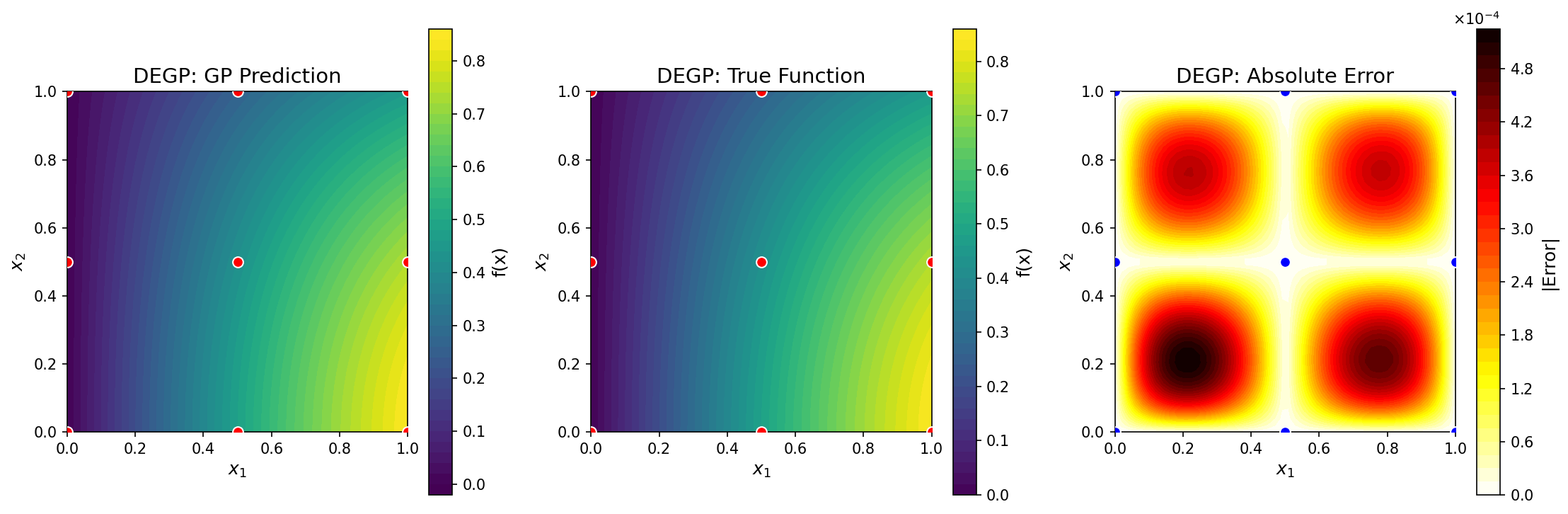
GP prediction (left), true function (center), and absolute error (right) for \(f(x_1, x_2) = \sin(x_1)\cos(x_2)\) using first and second-order coordinate-wise partial derivatives at nine regularly-spaced training points.#
—
DDEGP: Directional Derivative-Enhanced Gaussian Process#
DDEGP uses directional derivatives along global ray directions that are consistent across training points.
This example demonstrates DDEGP on the 2D function \(f(x_1, x_2) = x_1^2 + x_2^2\) using two global directional derivative directions applied at all training points.
Key feature: The rays parameter specifies global directions with shape (d, n_directions).
The derivative_locations parameter specifies which points have which directions.
import numpy as np
from jetgp.full_ddegp.ddegp import ddegp

# Generate 2D training data: f(x,y) = x^2 + y^2
np.random.seed(42)
X_train = np.random.rand(10, 2) * 2 - 1  # [-1, 1]^2
y_vals = np.sum(X_train**2, axis=1)
# Define two GLOBAL directional derivative directions
rays = np.array([
    [1.0, 0.5],   # x-components
    [0.0, 0.5]    # y-components
])

# Normalize direction vectors to unit length
for i in range(rays.shape[1]):
    rays[:, i] = rays[:, i] / np.linalg.norm(rays[:, i])

# derivative_locations: which points have which directions
# Here both directions at all 10 training points
num_pts = len(X_train)
derivative_locations = [
    list(range(num_pts)),  # Direction 1 at all points
    list(range(num_pts))   # Direction 2 at all points
]

# Compute directional derivatives: grad(f) · ray = 2*X · ray
dy_dray1 = np.sum(2*X_train * rays[:,0].reshape(1,-1), axis=1)
dy_dray2 = np.sum(2*X_train * rays[:,1].reshape(1,-1), axis=1)

Y_train = [y_vals.reshape(-1,1),
           dy_dray1.reshape(-1,1),
           dy_dray2.reshape(-1,1)]

# Specify directional derivative structure
der_indices = [[[[1,1]], [[2,1]]]]  # Two directions, first-order
# Initialize and optimize
model = ddegp(X_train, Y_train, n_order=1,
              der_indices=der_indices,
              derivative_locations=derivative_locations,
              rays=rays,
              normalize=True, kernel="SE",
              kernel_type="anisotropic")

params = model.optimize_hyperparameters(optimizer='lbfgs', n_restarts=5)
# Predict on grid
x_test = np.linspace(-1, 1, 50)
X1, X2 = np.meshgrid(x_test, x_test)
X_test = np.column_stack([X1.flatten(), X2.flatten()])

y_pred_full = model.predict(X_test, params, calc_cov=False, return_deriv=False)
y_pred = y_pred_full[0, :]  # Row 0: function values

# Compute error
y_true = np.sum(X_test**2, axis=1)
abs_error = np.abs(y_true - y_pred)

print(f"Mean absolute error: {np.mean(abs_error):.6f}")
print(f"Max absolute error: {np.max(abs_error):.6f}")
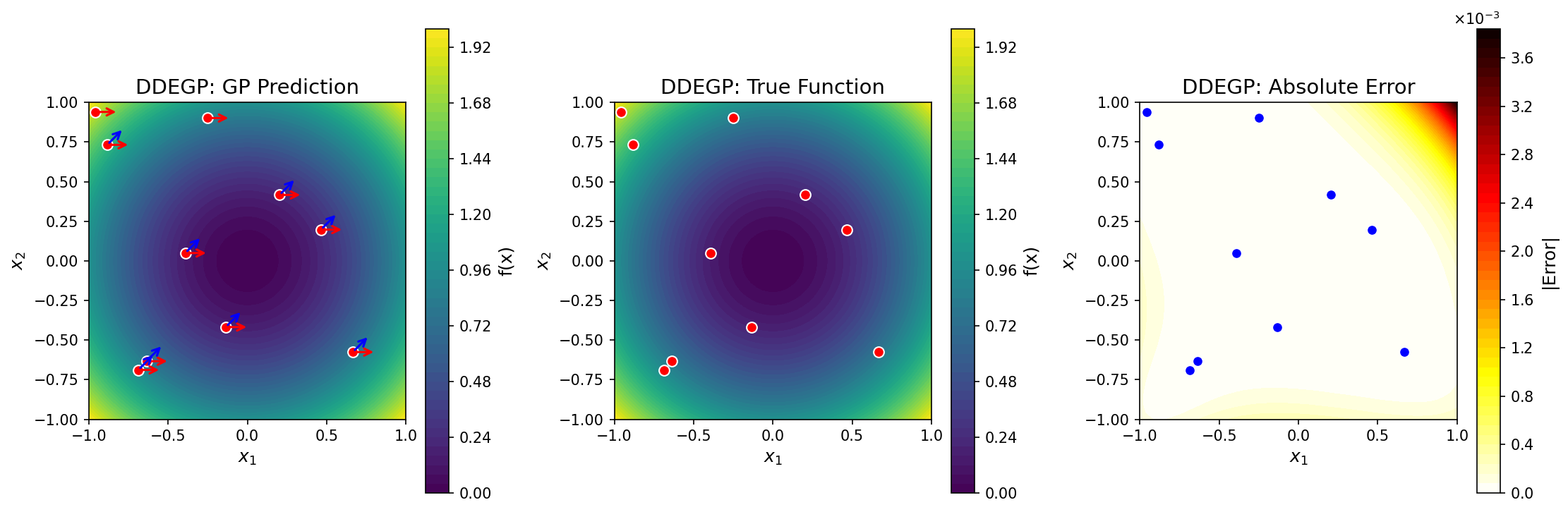
GP prediction (left), true function (center), and absolute error (right) for \(f(x_1, x_2) = x_1^2 + x_2^2\) using two global directional derivatives (shown as red and blue arrows) at ten randomly-placed training points. The directional rays are the same at all training locations.#
—
GDDEGP: Generalized Directional Derivative-Enhanced Gaussian Process#
GDDEGP uses point-wise directional derivatives where each training point can have unique ray directions.
This example demonstrates GDDEGP on the 2D function \(f(x_1, x_2) = x_1^2 + x_2^2\) using gradient-aligned and perpendicular directions that adapt to each location.
Key feature: The rays_list parameter contains arrays where rays_list[i][:, j] is the
ray direction for point derivative_locations[i][j]. Each column corresponds to a specific point.
import numpy as np
from jetgp.full_gddegp.gddegp import gddegp

# Generate 2D training data: f(x,y) = x^2 + y^2
np.random.seed(42)
X_train = np.random.rand(12, 2) * 2 - 1  # [-1, 1]^2
y_vals = np.sum(X_train**2, axis=1)
# Create POINT-WISE gradient and perpendicular directions
n_points = len(X_train)

# derivative_locations: all points have both directions
derivative_locations = [
    list(range(n_points)),  # Direction 1 at all points
    list(range(n_points))   # Direction 2 at all points
]

# Build rays_list: one array per direction
# rays_list[i][:, j] is the ray for point derivative_locations[i][j]
rays_dir1_list = []
rays_dir2_list = []

for i in range(n_points):
    # Gradient direction: [2x, 2y]
    gradient = 2 * X_train[i]
    grad_norm = np.linalg.norm(gradient)

    if grad_norm < 1e-10:
        ray1 = np.array([1.0, 0.0])
        ray2 = np.array([0.0, 1.0])
    else:
        # Direction 1: normalized gradient
        ray1 = gradient / grad_norm
        # Direction 2: perpendicular (rotate 90 degrees)
        ray2 = np.array([-ray1[1], ray1[0]])

    rays_dir1_list.append(ray1)
    rays_dir2_list.append(ray2)

rays_list = [
    np.column_stack(rays_dir1_list),  # Shape: (2, n_points)
    np.column_stack(rays_dir2_list)   # Shape: (2, n_points)
]
# Compute directional derivatives
dy_dray1 = np.array([np.dot(2*X_train[i], rays_list[0][:,i])
                     for i in range(n_points)])
dy_dray2 = np.array([np.dot(2*X_train[i], rays_list[1][:,i])
                     for i in range(n_points)])

y_train = [y_vals.reshape(-1,1),
           dy_dray1.reshape(-1,1),
           dy_dray2.reshape(-1,1)]

# der_indices: two first-order directional derivatives
der_indices = [[[[1,1]], [[2,1]]]]
# Initialize and optimize
model = gddegp(X_train, y_train, n_order=1,
               rays_list=rays_list,
               derivative_locations=derivative_locations,
               der_indices=der_indices,
               normalize=True, kernel="SE",
               kernel_type="anisotropic")

params = model.optimize_hyperparameters(optimizer='lbfgs', n_restarts=5)
# Predict on grid (no rays needed for function-only prediction)
x_test = np.linspace(-1, 1, 50)
X1, X2 = np.meshgrid(x_test, x_test)
X_test = np.column_stack([X1.flatten(), X2.flatten()])

y_pred_full = model.predict(X_test, params, calc_cov=False, return_deriv=False)
y_pred = y_pred_full[0, :]

# Compute error
y_true = np.sum(X_test**2, axis=1)
abs_error = np.abs(y_true - y_pred)

print(f"Mean absolute error: {np.mean(abs_error):.6f}")
print(f"Max absolute error: {np.max(abs_error):.6f}")
# Predict derivatives at training points (requires rays_predict)
y_pred_deriv = model.predict(
    X_train, params,
    rays_predict=rays_list,
    calc_cov=False,
    return_deriv=True
)

# Output shape: [3, n_points]
# Row 0: function values
# Row 1: Direction 1 derivatives
# Row 2: Direction 2 derivatives
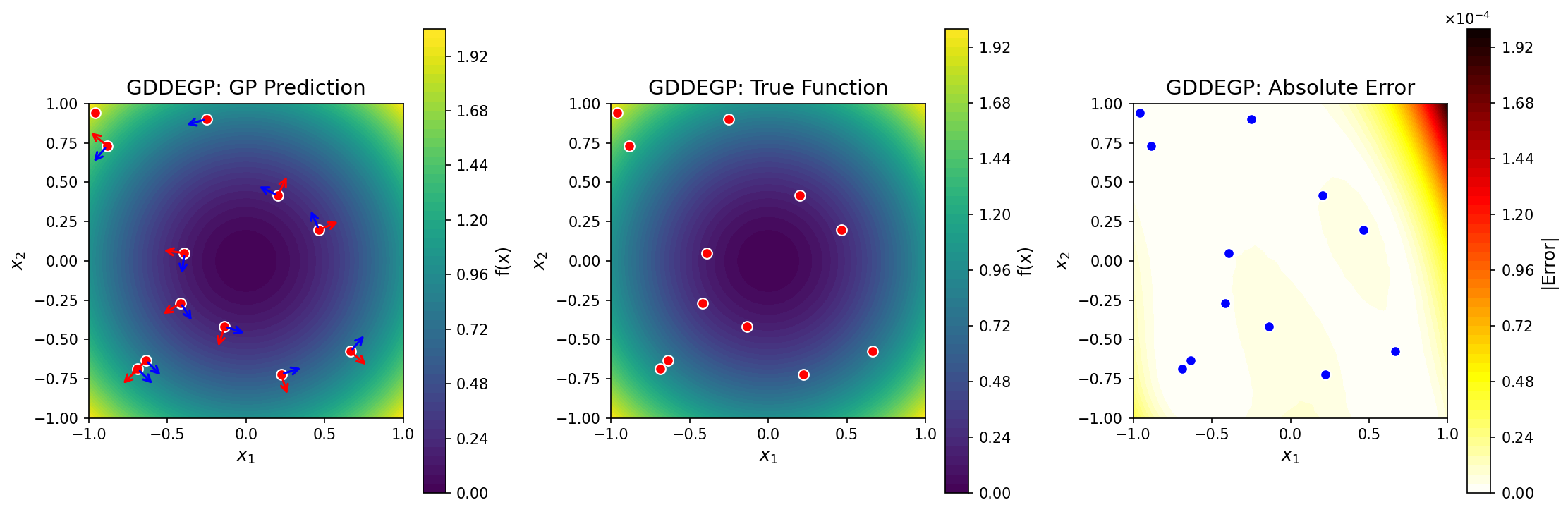
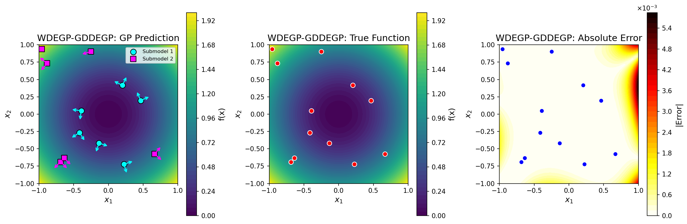
GP prediction (left), true function (center), and absolute error (right) for \(f(x_1, x_2) = x_1^2 + x_2^2\) using point-specific directional derivatives. At each training point, two orthogonal directions are used: one aligned with the local gradient (red arrows) and one perpendicular (blue arrows). Unlike DDEGP, the directions adapt to local function behavior.#
—
WDEGP: Weighted Derivative-Enhanced Gaussian Process#
WDEGP is a unified framework for combining multiple submodels trained on different subsets of
training points. It supports submodeling with any of the core module types through the
submodel_type parameter:
submodel_type='degp': Submodels use coordinate-aligned partial derivativessubmodel_type='ddegp': Submodels use global directional derivatives (requiresrays)submodel_type='gddegp': Submodels use point-wise directional derivatives (requiresrays_list)
Important: Derivative locations must be disjoint across submodels. If submodel 1 has derivative
information at point index i, submodel 2 cannot have derivative information at the same point.
Example 1: WDEGP with DEGP Submodels#
This example uses coordinate-aligned partial derivatives with two submodels on alternating points.
import numpy as np
from jetgp.wdegp.wdegp import wdegp

# Define test function: f(x) = sin(10*pi*x)/(2*x) + (x-1)^4
def f_fun(x):
    return np.sin(10*np.pi*x)/(2*x) + (x-1)**4

def f1_fun(x):  # First derivative
    return (10*np.pi*np.cos(10*np.pi*x))/(2*x) - \
           np.sin(10*np.pi*x)/(2*x**2) + 4*(x-1)**3

def f2_fun(x):  # Second derivative
    return -(100*np.pi**2*np.sin(10*np.pi*x))/(2*x) - \
           (20*np.pi*np.cos(10*np.pi*x))/(2*x**2) + \
           np.sin(10*np.pi*x)/(x**3) + 12*(x-1)**2

# Generate training points
X_train = np.linspace(0.5, 2.5, 10).reshape(-1, 1)

# Partition into DISJOINT submodels with alternating indices
submodel1_indices = [0, 2, 4, 6, 8]
submodel2_indices = [1, 3, 5, 7, 9]

# Function values at ALL training points
y_vals = f_fun(X_train.flatten()).reshape(-1, 1)
# Compute derivatives for each submodel at their specific indices
d1_sm1 = np.array([[f1_fun(X_train[i, 0])] for i in submodel1_indices])
d2_sm1 = np.array([[f2_fun(X_train[i, 0])] for i in submodel1_indices])
d1_sm2 = np.array([[f1_fun(X_train[i, 0])] for i in submodel2_indices])
d2_sm2 = np.array([[f2_fun(X_train[i, 0])] for i in submodel2_indices])

# Package submodel data
y_train = [
    [y_vals, d1_sm1, d2_sm1],  # Submodel 1
    [y_vals, d1_sm2, d2_sm2]   # Submodel 2
]

# Derivative locations: MUST be disjoint across submodels
derivative_locations = [
    [submodel1_indices, submodel1_indices],  # Submodel 1
    [submodel2_indices, submodel2_indices]   # Submodel 2
]

# Derivative specifications for each submodel
der_indices = [
    [[[[1, 1]]], [[[1, 2]]]],  # Submodel 1: 1st and 2nd order in dim 1
    [[[[1, 1]]], [[[1, 2]]]]   # Submodel 2: 1st and 2nd order in dim 1
]
# Initialize with submodel_type='degp' (default)
model = wdegp(X_train, y_train, n_order=2, n_bases=1,
              derivative_locations=derivative_locations,
              der_indices=der_indices,
              submodel_type='degp',
              normalize=True, kernel="SE",
              kernel_type="anisotropic")

params = model.optimize_hyperparameters(optimizer='jade',
                                        pop_size=100,
                                        n_generations=15)
# Predict with submodel outputs
X_test = np.linspace(0.5, 2.5, 250).reshape(-1, 1)
y_pred, y_cov, submodel_preds, submodel_covs = model.predict(
    X_test, params, calc_cov=True, return_submodels=True
)

# Compute error
y_true = f_fun(X_test.flatten())
abs_error = np.abs(y_true.flatten() - y_pred.flatten())

print(f"Mean absolute error: {np.mean(abs_error):.6f}")
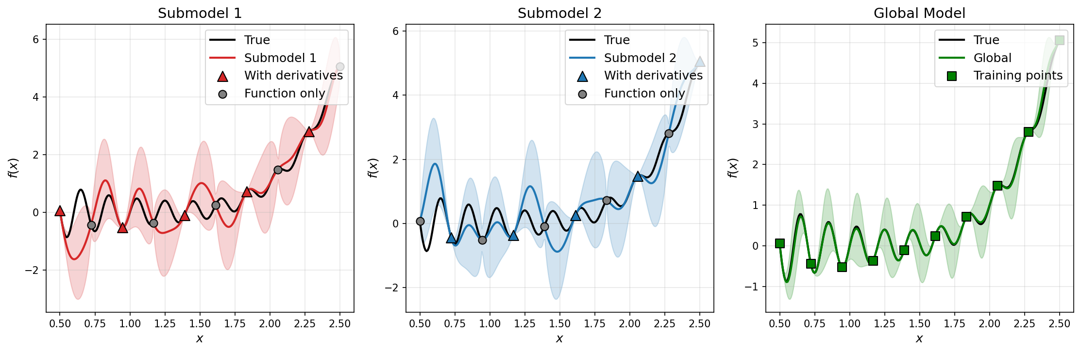
Comparison of submodel and global predictions for a 1D test function using DEGP submodels.#
Example 2: WDEGP with DDEGP Submodels#
This example uses global directional derivatives with two spatially-partitioned submodels.
import numpy as np
from jetgp.wdegp.wdegp import wdegp

# Generate 2D training data: f(x,y) = x^2 + y^2
np.random.seed(42)
X_train = np.random.rand(12, 2) * 2 - 1
y_vals = np.sum(X_train**2, axis=1).reshape(-1, 1)

# Define global rays (same at all points)
rays = np.array([
    [1.0, 0.0],   # x-components: ray1 along x, ray2 along y
    [0.0, 1.0]    # y-components
])

# DISJOINT submodels: left half vs right half
sm1_indices = [i for i in range(len(X_train)) if X_train[i, 0] < 0]
sm2_indices = [i for i in range(len(X_train)) if X_train[i, 0] >= 0]
# Compute directional derivatives for each submodel
dy_ray1_sm1 = (2 * X_train[sm1_indices, 0] * rays[0, 0] +
               2 * X_train[sm1_indices, 1] * rays[1, 0]).reshape(-1, 1)
dy_ray2_sm1 = (2 * X_train[sm1_indices, 0] * rays[0, 1] +
               2 * X_train[sm1_indices, 1] * rays[1, 1]).reshape(-1, 1)

dy_ray1_sm2 = (2 * X_train[sm2_indices, 0] * rays[0, 0] +
               2 * X_train[sm2_indices, 1] * rays[1, 0]).reshape(-1, 1)
dy_ray2_sm2 = (2 * X_train[sm2_indices, 0] * rays[0, 1] +
               2 * X_train[sm2_indices, 1] * rays[1, 1]).reshape(-1, 1)

y_train = [
    [y_vals, dy_ray1_sm1, dy_ray2_sm1],  # Submodel 1
    [y_vals, dy_ray1_sm2, dy_ray2_sm2]   # Submodel 2
]

der_indices = [
    [[[[1, 1]], [[2, 1]]]],  # Submodel 1: 2 directions
    [[[[1, 1]], [[2, 1]]]]   # Submodel 2: 2 directions
]

derivative_locations = [
    [sm1_indices, sm1_indices],  # Submodel 1
    [sm2_indices, sm2_indices]   # Submodel 2
]
# Initialize with submodel_type='ddegp'
model = wdegp(
    X_train, y_train, n_order=1, n_bases=2,
    der_indices=der_indices,
    derivative_locations=derivative_locations,
    submodel_type='ddegp',
    rays=rays,
    normalize=True, kernel="SE", kernel_type="anisotropic"
)

params = model.optimize_hyperparameters(
    optimizer='pso', pop_size=200, n_generations=15
)
# Predict
x_test = np.linspace(-1, 1, 50)
X1, X2 = np.meshgrid(x_test, x_test)
X_test = np.column_stack([X1.ravel(), X2.ravel()])

y_pred = model.predict(X_test, params, calc_cov=False)
y_true = np.sum(X_test**2, axis=1)

print(f"Mean absolute error: {np.mean(np.abs(y_true - y_pred.flatten())):.6f}")
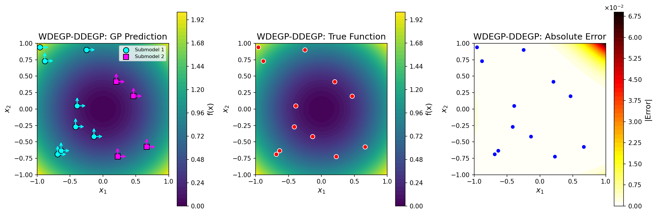
Comparison of submodel and global predictions for a 1D test function using DEGP submodels.#
Example 3: WDEGP with GDDEGP Submodels#
This example uses point-wise directional derivatives with gradient-aligned rays.
import numpy as np
from jetgp.wdegp.wdegp import wdegp

# Generate 2D training data: f(x,y) = x^2 + y^2
np.random.seed(42)
X_train = np.random.rand(12, 2) * 2 - 1
y_vals = np.sum(X_train**2, axis=1).reshape(-1, 1)

# DISJOINT submodels based on distance from origin
distances = np.linalg.norm(X_train, axis=1)
median_dist = np.median(distances)
sm1_indices = [i for i in range(len(X_train)) if distances[i] < median_dist]
sm2_indices = [i for i in range(len(X_train)) if distances[i] >= median_dist]
# Build point-wise rays for each submodel
def build_rays(indices):
    n = len(indices)
    rays_dir1 = np.zeros((2, n))
    rays_dir2 = np.zeros((2, n))
    dy_dir1 = np.zeros((n, 1))
    dy_dir2 = np.zeros((n, 1))

    for j, idx in enumerate(indices):
        grad = 2 * X_train[idx]
        grad_norm = np.linalg.norm(grad)

        if grad_norm < 1e-10:
            rays_dir1[:, j] = [1, 0]
            rays_dir2[:, j] = [0, 1]
        else:
            rays_dir1[:, j] = grad / grad_norm
            rays_dir2[:, j] = [-rays_dir1[1, j], rays_dir1[0, j]]

        dy_dir1[j] = np.dot(grad, rays_dir1[:, j])
        dy_dir2[j] = np.dot(grad, rays_dir2[:, j])

    return rays_dir1, rays_dir2, dy_dir1, dy_dir2

rays_dir1_sm1, rays_dir2_sm1, dy_dir1_sm1, dy_dir2_sm1 = build_rays(sm1_indices)
rays_dir1_sm2, rays_dir2_sm2, dy_dir1_sm2, dy_dir2_sm2 = build_rays(sm2_indices)

# rays_list: one entry per submodel, containing rays for each direction
rays_list = [
    [rays_dir1_sm1, rays_dir2_sm1],  # Submodel 1
    [rays_dir1_sm2, rays_dir2_sm2]   # Submodel 2
]

y_train = [
    [y_vals, dy_dir1_sm1, dy_dir2_sm1],
    [y_vals, dy_dir1_sm2, dy_dir2_sm2]
]

der_indices = [
    [[[[1, 1]], [[2, 1]]]],
    [[[[1, 1]], [[2, 1]]]]
]

derivative_locations = [
    [sm1_indices, sm1_indices],
    [sm2_indices, sm2_indices]
]
# Initialize with submodel_type='gddegp'
model = wdegp(
    X_train, y_train, n_order=1, n_bases=2,
    der_indices=der_indices,
    derivative_locations=derivative_locations,
    submodel_type='gddegp',
    rays_list=rays_list,
    normalize=True, kernel="SE", kernel_type="anisotropic"
)

params = model.optimize_hyperparameters(
    optimizer='pso', pop_size=200, n_generations=15
)
# Predict (function values only - no rays_predict needed)
x_test = np.linspace(-1, 1, 50)
X1, X2 = np.meshgrid(x_test, x_test)
X_test = np.column_stack([X1.ravel(), X2.ravel()])

y_pred = model.predict(X_test, params, calc_cov=False)
y_true = np.sum(X_test**2, axis=1)

print(f"Mean absolute error: {np.mean(np.abs(y_true - y_pred.flatten())):.6f}")
# Predict derivatives at training points (requires rays_predict)
# Build rays_predict for all training points
rays_dir1_all = np.zeros((2, len(X_train)))
rays_dir2_all = np.zeros((2, len(X_train)))

for j, idx in enumerate(sm1_indices):
    rays_dir1_all[:, idx] = rays_dir1_sm1[:, j]
    rays_dir2_all[:, idx] = rays_dir2_sm1[:, j]
for j, idx in enumerate(sm2_indices):
    rays_dir1_all[:, idx] = rays_dir1_sm2[:, j]
    rays_dir2_all[:, idx] = rays_dir2_sm2[:, j]

rays_predict = [rays_dir1_all, rays_dir2_all]

y_pred_deriv, _ = model.predict(
    X_train, params,
    rays_predict=rays_predict,
    calc_cov=True,
    return_deriv=True
)
## License
This project is licensed under the MIT License. See the LICENSE file for details.
Quick Access#
Theory of derivative-enhanced Gaussian Processes implemented in JetGP
Modules and minimal examples for using JetGP optimal step size selection algorithms.
Numerical examples showcasing JetGP capabilities