Sparse Derivative-Enhanced GP Tutorial: 2D Example#
This tutorial demonstrates a 2D sparse, derivative-enhanced Gaussian Process (DEGP) model using pyOTI-based automatic differentiation. It focuses on constructing a small 2D grid, strategically assigning derivative points, and visualizing model accuracy.
Key features#
2D grid-based training data generation
Non-contiguous index support: No reordering needed for derivative placement
Automatic differentiation using pyOTI
Contour visualization of the true function, GP prediction, and error
Highlighting of derivative points in the plots
Note
This example uses the Six-Hump Camelback function as a test case.
—
Import required packages#
import numpy as np
import itertools
import matplotlib.pyplot as plt
import pyoti.sparse as oti
from jetgp.wdegp.wdegp import wdegp
import jetgp.utils as utils
—
Configuration#
All configuration parameters are defined as simple variables. This includes derivative order, kernel type, and other hyperparameters.
n_order = 2
n_bases = 2
normalize_data = True
kernel = "SE"
kernel_type = "anisotropic"
n_restarts = 15
swarm_size = 200
np.random.seed(42)
Define the Six-Hump Camelback function#
def six_hump_camelback(X, alg=np):
    """
    Six-hump camelback function, a 2D benchmark function with multiple local minima.
    """
    x1 = X[:, 0]
    x2 = X[:, 1]
    return (
        (4 - 2.1 * x1**2 + (x1**4) / 3.0) * x1**2
        + x1 * x2
        + (-4 + 4 * x2**2) * x2**2
    )
—
Generate 2D training grid and derivative point assignment#
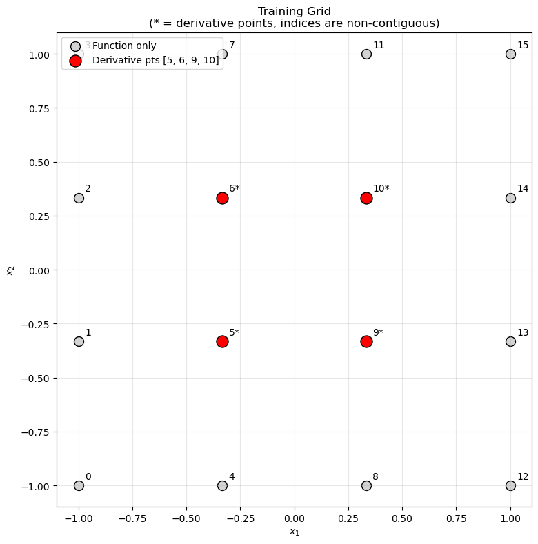
We construct a \(4 \times 4\) grid and select interior points for derivative computation.
No reordering needed! WDEGP supports non-contiguous indices, so we can use the interior point indices directly.
def create_training_grid(lb=-1.0, ub=1.0, num_points=4):
    """
    Create a 2D training grid with derivatives at interior points.

    No reordering needed - indices can be non-contiguous!
    """
    # Uniform 2D grid
    x_vals = np.linspace(lb, ub, num_points)
    y_vals = np.linspace(lb, ub, num_points)
    X = np.array(list(itertools.product(x_vals, y_vals)))

    # Interior points where we want derivatives (no reordering needed!)
    # In a 4x4 grid, interior points are [5, 6, 9, 10]
    derivative_indices = [5, 6, 9, 10]

    # Build submodel_indices structure:
    # submodel_indices[submodel][deriv_idx] = [list of point indices]
    # We have 4 derivatives total (2 dims × 2 orders), so 4 entries
    num_derivatives = n_bases * n_order  # 2 × 2 = 4
    submodel_indices = [
        [derivative_indices for _ in range(num_derivatives)]
    ]

    # Build derivative_specs structure:
    # derivative_specs[submodel][deriv_idx] = derivative spec
    # For 2D with all derivatives (4 total):
    derivative_specs = [
     [
         [[[1, 1]], [[2, 1]]],  # 1st order derivatives
         [[[1, 2]], [[2, 2]]]   # 2nd order derivatives
     ]
     ]

    return X, submodel_indices, derivative_specs, derivative_indices

X_train, submodel_indices, derivative_specs, derivative_indices = create_training_grid()

print(f"Total training points: {len(X_train)}")
print(f"Derivative indices (non-contiguous): {derivative_indices}")
print(f"\nsubmodel_indices: {len(submodel_indices[0])} entries (one per derivative)")
print(f"\nderivative_specs:")
deriv_names = ["df/dx1", "df/dx2", "d2f/dx1^2", "d2f/dx2^2"]
for i, spec in enumerate(derivative_specs[0]):
    print(f"  [{i}] {deriv_names[i]}: {spec}")
Total training points: 16
Derivative indices (non-contiguous): [5, 6, 9, 10]

submodel_indices: 4 entries (one per derivative)

derivative_specs:
  [0] df/dx1: [[[1, 1]], [[2, 1]]]
  [1] df/dx2: [[[1, 2]], [[2, 2]]]
Data structure explanation:
submodel_indices[0]has 4 entries (one per derivative)submodel_indices[0][i] = [5, 6, 9, 10]: Point indices for derivativeiderivative_specs[0][i]: The derivative specification for derivativei
Data structure explanation:
submodel_indices[0][0] = [5, 6, 9, 10]: 1st order derivatives at these pointssubmodel_indices[0][1] = [5, 6, 9, 10]: 2nd order derivatives at same pointsderivative_specs[0][0] = [[[1,1]], [[2,1]]]: 1st order specs (df/dx1, df/dx2)derivative_specs[0][1] = [[[1,2]], [[2,2]]]: 2nd order specs (d²f/dx1², d²f/dx2²)
—
Visualize grid and derivative points#
def visualize_grid(X_train, derivative_indices, lb=-1.0, ub=1.0):
    """Visualize the training grid with derivative points highlighted."""
    fig, ax = plt.subplots(figsize=(8, 8))

    # All points
    ax.scatter(X_train[:, 0], X_train[:, 1],
               c='lightgray', s=100, edgecolor='k', label='Function only')

    # Derivative points (non-contiguous indices!)
    ax.scatter(X_train[derivative_indices, 0], X_train[derivative_indices, 1],
               c='red', s=150, edgecolor='k', label=f'Derivative pts {derivative_indices}')

    # Label all points with their index
    for i, p in enumerate(X_train):
        label = f"{i}*" if i in derivative_indices else str(i)
        ax.text(p[0] + 0.03, p[1] + 0.03, label, fontsize=10)

    ax.set_title("Training Grid\n(* = derivative points, indices are non-contiguous)")
    ax.set_xlabel("$x_1$")
    ax.set_ylabel("$x_2$")
    ax.legend(loc='upper left')
    ax.grid(True, alpha=0.3)
    ax.set_aspect('equal')

    plt.tight_layout()
    plt.show()

visualize_grid(X_train, derivative_indices)
—
Prepare training data with derivatives#
def prepare_training_data(X_train, submodel_indices, derivative_specs, func, n_order=2):
    """
    Prepare function values and derivatives for WDEGP.

    Returns:
        submodel_data: List of [func_values, deriv_0, deriv_1, ...]
        where each deriv corresponds to one entry in derivative_specs
    """
    # Function values at ALL training points
    y_function_values = func(X_train, alg=np).reshape(-1, 1)

    submodel_data = []

    for k, (sm_indices, sm_deriv_specs) in enumerate(zip(submodel_indices, derivative_specs)):
        # Get the point indices for derivatives (same for all derivs in this example)
        point_indices = sm_indices[0]

        # Create OTI array for automatic differentiation
        X_sub = oti.array(X_train[point_indices])

        # Add OTI dual components for each dimension
        for dim in range(n_bases):
            for j in range(X_sub.shape[0]):
                X_sub[j, dim] += oti.e(dim + 1, order=n_order)

        # Evaluate function with OTI to get derivatives automatically
        y_with_derivs = oti.array([
            func(x, alg=oti)[0] for x in X_sub
        ])

        # Build submodel data: [func_values, deriv_0, deriv_1, ...]
        # Each derivative corresponds to one entry in derivative_specs
        current_data = [y_function_values]

        # Extract derivatives for each order
        for order_idx, order_specs in enumerate(sm_deriv_specs):
             for deriv_spec in order_specs:
                 deriv_values = y_with_derivs.get_deriv(deriv_spec).reshape(-1, 1)
                 current_data.append(deriv_values)

        submodel_data.append(current_data)

        print(f"Submodel {k} data structure:")
        print(f"  Function values: shape {current_data[0].shape} (all {len(X_train)} points)")
        deriv_names = ["df/dx1", "df/dx2", "d2f/dx1^2", "d2f/dx2^2"]
        for idx, arr in enumerate(current_data[1:]):
            print(f"  [{idx}] {deriv_names[idx]}: shape {arr.shape} ({len(point_indices)} points)")

    return submodel_data

submodel_data = prepare_training_data(
    X_train, submodel_indices, derivative_specs, six_hump_camelback, n_order
)
print(f"\nTotal submodels: {len(submodel_data)}")
print(f"Arrays per submodel: {len(submodel_data[0])}")
Submodel 0 data structure:
  Function values: shape (16, 1) (all 16 points)
  [0] df/dx1: shape (4, 1) (4 points)
  [1] df/dx2: shape (4, 1) (4 points)
  [2] d2f/dx1^2: shape (4, 1) (4 points)
  [3] d2f/dx2^2: shape (4, 1) (4 points)

Total submodels: 1
Arrays per submodel: 5
—
Build and optimize the GP model#
print("Building WDEGP model...")
print(f"  Training points: {len(X_train)}")
print(f"  Derivative points: {len(derivative_indices)} (at indices {derivative_indices})")
print(f"  Derivatives per point: {n_bases * n_order} (2 dims × 2 orders)")

gp_model = wdegp(
    X_train,
    submodel_data,
    n_order,
    n_bases,
    derivative_specs,
    derivative_locations = submodel_indices,
    normalize=normalize_data,
    kernel=kernel,
    kernel_type=kernel_type,
)

print("\nOptimizing hyperparameters...")
params = gp_model.optimize_hyperparameters(
    optimizer='jade',
    pop_size=100,
    n_generations=15,
    local_opt_every=None,
    debug=True
)

print("\nOptimized parameters:")
print(params)
Building WDEGP model...
  Training points: 16
  Derivative points: 4 (at indices [5, 6, 9, 10])
  Derivatives per point: 4 (2 dims × 2 orders)

Optimizing hyperparameters...
Gen 1: best f=47.91385918475584
Gen 2: best f=18.045345256799862
Gen 3: best f=18.045345256799862
Gen 4: best f=18.045345256799862
Gen 5: best f=15.348355135768827
Gen 6: best f=15.348355135768827
Gen 7: best f=15.348355135768827
Gen 8: best f=13.233077630609856
Gen 9: best f=11.936236154792113
Gen 10: best f=11.936236154792113
Gen 11: best f=11.516952793850749
Gen 12: best f=11.516952793850749
Gen 13: best f=11.516952793850749
Gen 14: best f=11.516952793850749
Gen 15: best f=11.516952793850749

Optimized parameters:
[ -0.26883153  -0.09019859   0.94748321 -14.09571385]
—
Evaluate model performance on test grid#
def evaluate_gp(gp_model, func, params, lb=-1.0, ub=1.0, N=50):
    """Evaluate GP on a dense test grid."""
    x_lin = np.linspace(lb, ub, N)
    y_lin = np.linspace(lb, ub, N)
    X1, X2 = np.meshgrid(x_lin, y_lin)
    X_test = np.column_stack([X1.ravel(), X2.ravel()])

    y_pred = gp_model.predict(X_test, params, calc_cov=False)
    y_true = func(X_test, alg=np)

    # Error metrics
    rmse = np.sqrt(np.mean((y_true - y_pred.flatten())**2))
    nrmse = rmse / (y_true.max() - y_true.min())
    mae = np.mean(np.abs(y_true - y_pred.flatten()))

    return X1, X2, y_true.reshape(N, N), y_pred.reshape(N, N), nrmse, rmse, mae

X1, X2, y_true_grid, y_pred_grid, nrmse, rmse, mae = evaluate_gp(
    gp_model, six_hump_camelback, params
)
print(f"NRMSE: {nrmse:.6f}")
print(f"RMSE:  {rmse:.6f}")
print(f"MAE:   {mae:.6f}")
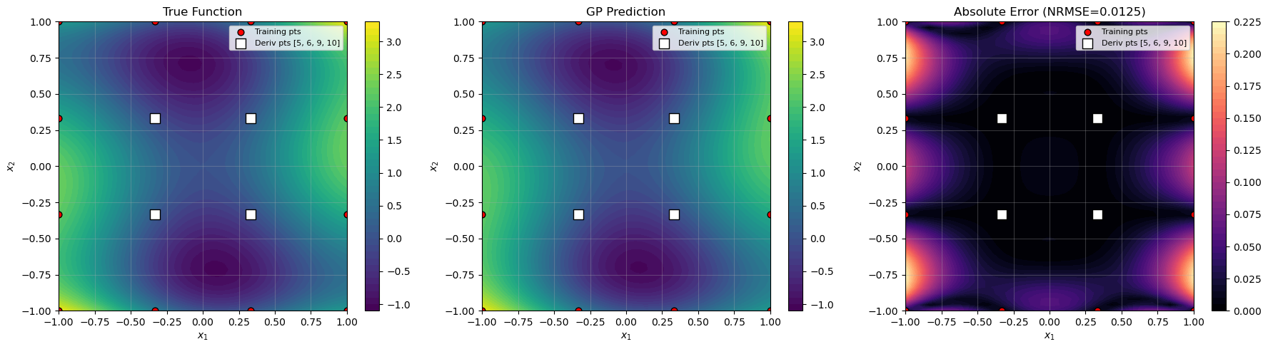
NRMSE: 0.012538
RMSE:  0.053467
MAE:   0.034333
—
Visualize results#
def visualize_results(X1, X2, y_true, y_pred, X_train, derivative_indices, nrmse):
    """Create contour plots of true function, prediction, and error."""
    abs_err = np.abs(y_true - y_pred)
    fig, axes = plt.subplots(1, 3, figsize=(18, 5))

    titles = ["True Function", "GP Prediction", f"Absolute Error (NRMSE={nrmse:.4f})"]
    data = [y_true, y_pred, abs_err]
    cmaps = ["viridis", "viridis", "magma"]

    for ax, Z, title, cmap in zip(axes, data, titles, cmaps):
        c = ax.contourf(X1, X2, Z, levels=50, cmap=cmap)
        fig.colorbar(c, ax=ax)

        # All training points
        ax.scatter(X_train[:, 0], X_train[:, 1],
                   c='red', edgecolor='k', s=40, label='Training pts')

        # Derivative points (highlighted)
        ax.scatter(X_train[derivative_indices, 0], X_train[derivative_indices, 1],
                   c='white', edgecolor='k', s=100, marker='s',
                   label=f'Deriv pts {derivative_indices}')

        ax.set_title(title)
        ax.set_xlabel("$x_1$")
        ax.set_ylabel("$x_2$")
        ax.legend(loc='upper right', fontsize=8)
        ax.grid(alpha=0.3)

    plt.tight_layout()
    plt.show()

visualize_results(X1, X2, y_true_grid, y_pred_grid, X_train, derivative_indices, nrmse)
—
Verify derivative interpolation#
Since this is a single submodel, return_deriv=True is available for direct derivative predictions.
print("=" * 70)
print("Derivative verification using return_deriv=True")
print("=" * 70)

# Get predictions with derivatives at the derivative training points
X_deriv_pts = X_train[derivative_indices]
y_pred_with_derivs = gp_model.predict(X_deriv_pts, params, calc_cov=False, return_deriv=True)

print(f"\nPrediction shape: {y_pred_with_derivs.shape}")
print("  Row 0: function values")
print("  Row 1: df/dx1 (1st order, dim 1)")
print("  Row 2: df/dx2 (1st order, dim 2)")
print("  Row 3: d²f/dx1² (2nd order, dim 1)")
print("  Row 4: d²f/dx2² (2nd order, dim 2)")

# Compare with training data
print("\n1st order derivatives (df/dx1):")
pred_d1_x1 = y_pred_with_derivs[1, :]
true_d1_x1 = submodel_data[0][1].flatten()  # 1st deriv array
for i, idx in enumerate(derivative_indices):
    rel_err = abs(pred_d1_x1[i] - true_d1_x1[i]) / abs(true_d1_x1[i]) if true_d1_x1[i] != 0 else 0
    print(f"  Point {idx}: Pred={pred_d1_x1[i]:.6f}, True={true_d1_x1[i]:.6f}, RelErr={rel_err:.2e}")

print("\n1st order derivatives (df/dx2):")
pred_d1_x2 = y_pred_with_derivs[2, :]
true_d1_x2 = submodel_data[0][2].flatten()
for i, idx in enumerate(derivative_indices):
    rel_err = abs(pred_d1_x2[i] - true_d1_x2[i]) / abs(true_d1_x2[i]) if true_d1_x2[i] != 0 else 0
    print(f"  Point {idx}: Pred={pred_d1_x2[i]:.6f}, True={true_d1_x2[i]:.6f}, RelErr={rel_err:.2e}")
======================================================================
Derivative verification using return_deriv=True
======================================================================
Making predictions for all derivatives that are common among submodels

Prediction shape: (5, 4)
  Row 0: function values
  Row 1: df/dx1 (1st order, dim 1)
  Row 2: df/dx2 (1st order, dim 2)
  Row 3: d²f/dx1² (2nd order, dim 1)
  Row 4: d²f/dx2² (2nd order, dim 2)

1st order derivatives (df/dx1):
  Point 5: Pred=5.323457, True=-2.697119, RelErr=2.97e+00
  Point 6: Pred=5.323457, True=-2.030453, RelErr=3.62e+00
  Point 9: Pred=5.323457, True=2.030453, RelErr=1.62e+00
  Point 10: Pred=5.323457, True=2.697119, RelErr=9.74e-01

1st order derivatives (df/dx2):
  Point 5: Pred=-2.697119, True=1.740741, RelErr=2.55e+00
  Point 6: Pred=-2.030453, True=-2.407407, RelErr=1.57e-01
  Point 9: Pred=2.030453, True=2.407407, RelErr=1.57e-01
  Point 10: Pred=2.697119, True=-1.740741, RelErr=2.55e+00
—
Summary#
This tutorial demonstrated a 2D sparse DEGP model with selective derivative placement.
Key features:
No reordering needed: Non-contiguous indices (
[5, 6, 9, 10]) are used directlyInterior derivative points: Derivatives at interior grid points improve accuracy in nonlinear regions
Direct derivative verification:
return_deriv=Trueprovides predicted derivatives
Data structures used:
# submodel_indices[submodel][deriv_idx] = [point indices]
# One entry per derivative (4 total for 2D × 2 orders)
submodel_indices = [
    [d_indices, d_indices, d_indices, d_indices]
]

# derivative_specs[submodel][deriv_idx] = derivative spec
derivative_specs = [
    [
        [[[1, 1]]],  # df/dx1
        [[[2, 1]]],  # df/dx2
        [[[1, 2]]],  # d²f/dx1²
        [[[2, 2]]]   # d²f/dx2²
    ]
]
Advantages:
Efficient use of derivative information at strategic locations
No data reorganization required
Direct access to derivative predictions via
return_deriv=True