High-Dimensional DEGP Tutorial: 4D Function Approximation with 2D Visualization

High-Dimensional DEGP Tutorial: 4D Function Approximation with 2D Visualization#

In this tutorial, Derivative-Enhanced Gaussian Processes (DEGPs) are applied to a high-dimensional 4D function. We analyze the model’s performance through 2D slices of the input space, which allows us to visualize complex high-dimensional behavior in a comprehensible way.

This approach is useful for: - Understanding the behavior of high-dimensional nonlinear functions. - Leveraging derivative information to improve model accuracy. - Reducing computational cost by selectively including key derivatives.

Setup #

We begin by importing all necessary libraries, including pyoti for hypercomplex AD, full_degp for DEGP modeling, and standard scientific Python packages.

import numpy as np
import pyoti.sparse as oti
from jetgp.full_degp.degp import degp
import jetgp.utils as utils
import time
from matplotlib import pyplot as plt
from scipy.stats import qmc
from typing import List, Dict, Callable

Configuration #

We explicitly define all configuration parameters as simple variables. This includes the dimensionality of the input space, number of training points, kernel type, and other hyperparameters.

n_bases = 4
n_order = 2
num_training_pts = 25
slice_grid_resolution = 25
lower_bounds = [-5.0]*4
upper_bounds = [5.0]*4
normalize_data = True
kernel = "SE"
kernel_type = "anisotropic"
n_restarts = 15
swarm_size = 200
random_seed = 1354
np.random.seed(random_seed)

True Function #

The function we aim to model is the 4D Styblinski–Tang function. It is nonlinear and exhibits multiple minima, making it a challenging test case for high-dimensional regression methods.

def styblinski_tang_4d(X, alg=oti):
    """
    Styblinski–Tang function in 4D:
    f(x1,x2,x3,x4) = 0.5 * sum_{i=1}^4 (x_i^4 - 16 x_i^2 + 5 x_i)
    """
    x1, x2, x3, x4 = X[:,0], X[:,1], X[:,2], X[:,3]
    return 0.5 * (x1**4 - 16*x1**2 + 5*x1 +
                  x2**4 - 16*x2**2 + 5*x2 +
                  x3**4 - 16*x3**2 + 5*x3 +
                  x4**4 - 16*x4**2 + 5*x4)

Derivative Strategy #

DEGP allows us to include derivative observations to improve the predictive accuracy of the model. Here we select only the main first- and second-order derivatives, which significantly reduces computational cost while preserving accuracy.

def analyze_derivatives(n_bases, n_order):
    """Select main derivatives only (1st and 2nd order) and print counts."""
    complete_indices = utils.gen_OTI_indices(n_bases, n_order)
    complete_count = sum(len(group) for group in complete_indices)

    der_indices = [
        [[[i + 1, 1]] for i in range(n_bases)],  # 1st order
        [[[i + 1, 2]] for i in range(n_bases)]   # 2nd order
    ]
    selective_count = sum(len(group) for group in der_indices)

    print(f"Complete derivative set: {complete_count} terms (incl. cross-terms)")
    print(f"Selective strategy: {selective_count} terms (main derivatives only)")
    print(f"Reduction factor: {complete_count/selective_count:.1f}x")
    return der_indices

Training Data Generation #

We generate training data using Sobol sequences to efficiently cover the high-dimensional space. For each training point, we evaluate the function as well as the selected derivatives. We also construct the derivative_locations list to specify that all derivatives are available at all training points.

def generate_training_data(n_bases, n_order, num_training_pts, lower_bounds, upper_bounds, der_indices):
    sampler = qmc.Sobol(d=n_bases, scramble=True, seed=42)
    sobol_sample = sampler.random_base2(m=int(np.ceil(np.log2(num_training_pts))))
    X_train = utils.scale_samples(sobol_sample, lower_bounds, upper_bounds)

    X_train_pert = oti.array(X_train)
    for i in range(n_bases):
        X_train_pert[:, i] += oti.e(i+1, order=n_order)

    y_train_hc = styblinski_tang_4d(X_train_pert)
    y_train_list = [y_train_hc.real]
    for group in der_indices:
        for sub_group in group:
            y_train_list.append(y_train_hc.get_deriv(sub_group))

    # Build derivative_locations: one entry per derivative, all at all points
    derivative_locations = []
    for i in range(len(der_indices)):
        for j in range(len(der_indices[i])):
            derivative_locations.append([k for k in range(len(X_train))])

    print(f"Total observations: {sum(d.shape[0] for d in y_train_list)}")
    print(f"Derivative locations: {len(derivative_locations)} entries, each with {len(X_train)} points")
    return X_train, y_train_list, derivative_locations

Model Training #

We initialize the DEGP model and optimize its hyperparameters using JADE optimization. The model incorporates both function values and selected derivatives, with derivative_locations specifying where each derivative is available.

def train_model(X_train, y_train_list, n_order, n_bases, der_indices, derivative_locations, normalize_data, kernel, kernel_type, n_restarts, swarm_size):
    gp_model = degp(
        X_train, y_train_list, n_order, n_bases,
        der_indices,
        derivative_locations=derivative_locations,
        normalize=normalize_data,
        kernel=kernel, kernel_type=kernel_type
    )
    params = gp_model.optimize_hyperparameters(
        optimizer='pso',
        pop_size=250,
        n_generations=30,
        local_opt_every=30,
        debug=True
    )
    return gp_model, params

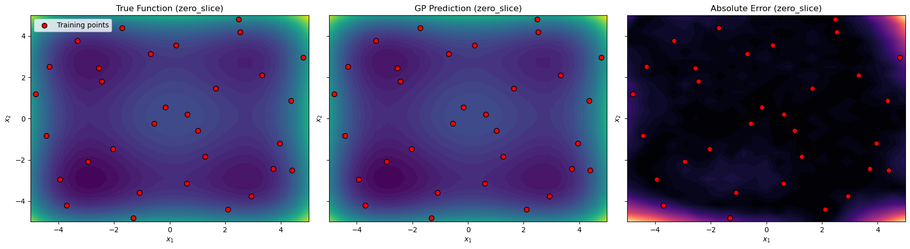
2D Slice Evaluation #

To visualize high-dimensional behavior, we evaluate the model on 2D slices of the 4D space. Here, the remaining two dimensions are fixed at zero, the domain center, or a random point.

def evaluate_slice(X_test_fixed_values):
    x_lin = np.linspace(lower_bounds[0], upper_bounds[0], slice_grid_resolution)
    y_lin = np.linspace(lower_bounds[1], upper_bounds[1], slice_grid_resolution)
    X1_grid, X2_grid = np.meshgrid(x_lin, y_lin)

    X_test = np.zeros((X1_grid.size, n_bases))
    X_test[:,0] = X1_grid.ravel()
    X_test[:,1] = X2_grid.ravel()
    for i, val in enumerate(X_test_fixed_values):
        X_test[:, i+2] = val

    y_pred, y_var = gp_model.predict(X_test, params, calc_cov=True)
    y_true = styblinski_tang_4d(X_test, alg=np)

    return {
        "X1_grid": X1_grid, "X2_grid": X2_grid,
        "y_true": y_true.reshape(X1_grid.shape),
        "y_pred": y_pred.reshape(X1_grid.shape),
        "nrmse": utils.nrmse(y_true, y_pred)
    }

Visualization #

We create contour plots of the true function, the GP prediction, and the absolute error for each 2D slice. Training points are overlaid to show their locations relative to the evaluation grid.

def plot_slices(X_train, slice_results, slice_name="zero_slice"):
    fig, axes = plt.subplots(1,3, figsize=(18,5), sharex=True, sharey=True)
    X_train_proj = X_train[:,:2]

    # True function
    axes[0].contourf(slice_results["X1_grid"], slice_results["X2_grid"], slice_results["y_true"], levels=50, cmap="viridis")
    axes[0].scatter(X_train_proj[:,0], X_train_proj[:,1], c="red", edgecolor="k", s=50, label="Training points")
    axes[0].set_title(f"True Function ({slice_name})")
    axes[0].legend()

    # GP prediction
    axes[1].contourf(slice_results["X1_grid"], slice_results["X2_grid"], slice_results["y_pred"], levels=50, cmap="viridis")
    axes[1].scatter(X_train_proj[:,0], X_train_proj[:,1], c="red", edgecolor="k", s=50)
    axes[1].set_title(f"GP Prediction ({slice_name})")

    # Absolute error
    error_grid = np.abs(slice_results["y_true"] - slice_results["y_pred"])
    axes[2].contourf(slice_results["X1_grid"], slice_results["X2_grid"], error_grid, levels=50, cmap="magma")
    axes[2].scatter(X_train_proj[:,0], X_train_proj[:,1], c="red", edgecolor="k", s=50)
    axes[2].set_title(f"Absolute Error ({slice_name})")

    for ax in axes:
        ax.set_xlabel("$x_1$")
        ax.set_ylabel("$x_2$")
    plt.tight_layout()
    plt.show()

Full Workflow #

Finally, we run the full workflow: analyze derivatives, generate training data (including derivative locations), train the model, evaluate a zero slice, and visualize the results.

der_indices = analyze_derivatives(n_bases, n_order)
X_train, y_train_list, derivative_locations = generate_training_data(
    n_bases, n_order, num_training_pts,
    lower_bounds, upper_bounds, der_indices
)

gp_model, params = train_model(
    X_train, y_train_list, n_order, n_bases,
    der_indices, derivative_locations,
    normalize_data, kernel, kernel_type,
    n_restarts, swarm_size
)

# Evaluate a 2D slice with the last two dimensions fixed at zero
slice_results = evaluate_slice(X_test_fixed_values=[0.0, 0.0])

# Visualize the slice
plot_slices(X_train, slice_results, slice_name="zero_slice")

Complete derivative set: 14 terms (incl. cross-terms)
Selective strategy: 8 terms (main derivatives only)
Reduction factor: 1.8x
Total observations: 288
Derivative locations: 8 entries, each with 32 points

New best for swarm at iteration 1: [ 0.02279516  0.09497524  0.20586795  0.13493861  0.69434126 -5.72591109] 874.2092347793057

Best after iteration 1: [ 0.02279516  0.09497524  0.20586795  0.13493861  0.69434126 -5.72591109] 874.2092347793057

Best after iteration 2: [ 0.02279516  0.09497524  0.20586795  0.13493861  0.69434126 -5.72591109] 874.2092347793057

New best for swarm at iteration 3: [-0.78718021 -1.12060992 -0.42553376 -0.92708697  3.9714838  -4.58824157] 621.6753586048937
Best after iteration 3: [-0.78718021 -1.12060992 -0.42553376 -0.92708697  3.9714838  -4.58824157] 621.6753586048937

New best for swarm at iteration 4: [-0.44893226 -0.53510706 -0.31977985 -0.60563432  2.43884712 -6.03379599] 540.5113675556723

Best after iteration 4: [-0.44893226 -0.53510706 -0.31977985 -0.60563432  2.43884712 -6.03379599] 540.5113675556723
New best for swarm at iteration 5: [-0.74299303 -0.45405842 -0.54662726 -0.60357143  2.85565382 -4.63862817] 469.62291674984317

Best after iteration 5: [-0.74299303 -0.45405842 -0.54662726 -0.60357143  2.85565382 -4.63862817] 469.62291674984317
New best for swarm at iteration 6: [-0.42355832 -0.58898204 -0.4120302  -0.50087364  2.15387536 -5.21676809] 457.9643520004015

New best for swarm at iteration 6: [-0.96324501 -0.63163179 -0.9774898  -0.7407199   3.70552312 -4.90592171] 337.2796675429154

Best after iteration 6: [-0.96324501 -0.63163179 -0.9774898  -0.7407199   3.70552312 -4.90592171] 337.2796675429154
New best for swarm at iteration 7: [-0.74712778 -0.7286189  -0.63433269 -0.7614569   3.20941561 -4.93808471] 208.63685957002644

Best after iteration 7: [-0.74712778 -0.7286189  -0.63433269 -0.7614569   3.20941561 -4.93808471] 208.63685957002644

New best for swarm at iteration 8: [-0.76127503 -0.89763207 -0.84012454 -0.83224439  3.44273492 -5.09216471] 71.83881717448611

Best after iteration 8: [-0.76127503 -0.89763207 -0.84012454 -0.83224439  3.44273492 -5.09216471] 71.83881717448611

Best after iteration 9: [-0.76127503 -0.89763207 -0.84012454 -0.83224439  3.44273492 -5.09216471] 71.83881717448611
New best for swarm at iteration 10: [-0.87489507 -0.89054703 -0.95130521 -0.85262932  3.66588903 -4.65925444] 7.020581540348871
New best for swarm at iteration 10: [-0.91950448 -0.9454822  -0.87768264 -0.88474765  3.61768481 -4.88295262] -3.348287887725803

Best after iteration 10: [-0.91950448 -0.9454822  -0.87768264 -0.88474765  3.61768481 -4.88295262] -3.348287887725803
New best for swarm at iteration 11: [-0.87439975 -0.93464544 -0.90182491 -0.88809714  3.66604648 -4.88837615] -30.84156065329205

Best after iteration 11: [-0.87439975 -0.93464544 -0.90182491 -0.88809714  3.66604648 -4.88837615] -30.84156065329205
New best for swarm at iteration 12: [-0.88311934 -0.96414665 -0.90999153 -0.9074942   3.73515762 -4.2163338 ] -33.60708459982328

New best for swarm at iteration 12: [-0.88732138 -0.89684952 -0.92591259 -0.90168838  3.70264262 -4.978146  ] -39.3816241905115

New best for swarm at iteration 12: [-0.90741169 -0.91571044 -0.89118043 -0.90647772  3.73516103 -4.95239336] -45.53668389062511
Best after iteration 12: [-0.90741169 -0.91571044 -0.89118043 -0.90647772  3.73516103 -4.95239336] -45.53668389062511

Best after iteration 13: [-0.90741169 -0.91571044 -0.89118043 -0.90647772  3.73516103 -4.95239336] -45.53668389062511
New best for swarm at iteration 14: [-0.91859664 -0.91203348 -0.89035762 -0.92691109  3.73221197 -5.00417469] -49.59959596249308

New best for swarm at iteration 14: [-0.91157155 -0.94371369 -0.91250547 -0.92533144  3.7468499  -5.00242901] -61.02467265473581

Best after iteration 14: [-0.91157155 -0.94371369 -0.91250547 -0.92533144  3.7468499  -5.00242901] -61.02467265473581

Best after iteration 15: [-0.91157155 -0.94371369 -0.91250547 -0.92533144  3.7468499  -5.00242901] -61.02467265473581

New best for swarm at iteration 16: [-0.91300263 -0.93355415 -0.91590401 -0.9444548   3.75305492 -4.95316893] -62.12699075403856

New best for swarm at iteration 16: [-0.91085082 -0.94674931 -0.92124631 -0.91469877  3.76634682 -4.96106331] -62.62467820205859
Best after iteration 16: [-0.91085082 -0.94674931 -0.92124631 -0.91469877  3.76634682 -4.96106331] -62.62467820205859

New best for swarm at iteration 17: [-0.91477744 -0.94137399 -0.91944314 -0.92411918  3.76805883 -4.8699056 ] -65.57542556184632
New best for swarm at iteration 17: [-0.91425629 -0.94591591 -0.93043006 -0.92045518  3.80283456 -4.79105317] -66.87298408858163

Best after iteration 17: [-0.91425629 -0.94591591 -0.93043006 -0.92045518  3.80283456 -4.79105317] -66.87298408858163

New best for swarm at iteration 18: [-0.92513989 -0.94039804 -0.93068793 -0.91987628  3.76653176 -4.89777339] -67.75880455614703

Best after iteration 18: [-0.92513989 -0.94039804 -0.93068793 -0.91987628  3.76653176 -4.89777339] -67.75880455614703

Best after iteration 19: [-0.92513989 -0.94039804 -0.93068793 -0.91987628  3.76653176 -4.89777339] -67.75880455614703
New best for swarm at iteration 20: [-0.91922614 -0.94380459 -0.93450381 -0.92160133  3.77745838 -4.8785549 ] -69.63962279208596

Best after iteration 20: [-0.91922614 -0.94380459 -0.93450381 -0.92160133  3.77745838 -4.8785549 ] -69.63962279208596

Best after iteration 21: [-0.91922614 -0.94380459 -0.93450381 -0.92160133  3.77745838 -4.8785549 ] -69.63962279208596

Best after iteration 22: [-0.91922614 -0.94380459 -0.93450381 -0.92160133  3.77745838 -4.8785549 ] -69.63962279208596

Best after iteration 23: [-0.91922614 -0.94380459 -0.93450381 -0.92160133  3.77745838 -4.8785549 ] -69.63962279208596

Best after iteration 24: [-0.91922614 -0.94380459 -0.93450381 -0.92160133  3.77745838 -4.8785549 ] -69.63962279208596

Best after iteration 25: [-0.91922614 -0.94380459 -0.93450381 -0.92160133  3.77745838 -4.8785549 ] -69.63962279208596

Best after iteration 26: [-0.91922614 -0.94380459 -0.93450381 -0.92160133  3.77745838 -4.8785549 ] -69.63962279208596

Best after iteration 27: [-0.91922614 -0.94380459 -0.93450381 -0.92160133  3.77745838 -4.8785549 ] -69.63962279208596

New best for swarm at iteration 28: [-0.92141863 -0.94274298 -0.93289171 -0.92072218  3.77155469 -4.8859265 ] -70.19140378952335
Best after iteration 28: [-0.92141863 -0.94274298 -0.93289171 -0.92072218  3.77155469 -4.8859265 ] -70.19140378952335

Best after iteration 29: [-0.92141863 -0.94274298 -0.93289171 -0.92072218  3.77155469 -4.8859265 ] -70.19140378952335

Local optimization did not improve:
Best after iteration 30: [-0.92141863 -0.94274298 -0.93289171 -0.92072218  3.77155469 -4.8859265 ] -70.19140378952335
Stopping: maximum iterations reached --> 30
Warning: Cholesky decomposition failed via scipy, using standard np solve instead.

High-Dimensional DEGP Tutorial: 4D Function Approximation with 2D Visualization

Contents

High-Dimensional DEGP Tutorial: 4D Function Approximation with 2D Visualization#