Cycling Spatial Derivative Strategy for DEGP#
This tutorial demonstrates a spatially-aware derivative assignment strategy for Derivative-Enhanced Gaussian Processes (DEGPs). Instead of providing all derivatives at every training point, we assign exactly one derivative per point, cycling through dimensions along a spatial chain.
This approach is useful for:
Reducing computational cost in high-dimensional problems.
Exploring trade-offs between derivative coverage and model accuracy.
Understanding how GP correlation structure propagates derivative information.
Motivation#
In high-dimensional problems, providing full derivative information at every training point can be computationally expensive. The covariance matrix size scales with the total number of observations, so reducing derivative observations can significantly improve training time and memory usage.
Key insight: Gaussian Processes have a correlation structure that allows nearby points to share information. If neighboring points have complementary derivative information, the GP may be able to “fill in” the missing derivatives through spatial correlation.
The Strategy#
The cycling derivative strategy works as follows:
Build a spatial chain: Connect training points via a nearest-neighbor path
Cycle derivatives along the chain: Assign derivatives in a repeating pattern
For a 2D problem:
Position 0, 2, 4, … → ∂f/∂x₁
Position 1, 3, 5, … → ∂f/∂x₂
This ensures that adjacent points in the chain have different derivative information, maximizing the complementary coverage.
Setup#
We begin by importing all necessary libraries, including pyoti for hypercomplex
AD, full_degp for DEGP modeling, and standard scientific Python packages.
import numpy as np
import pyoti.sparse as oti
from jetgp.full_degp.degp import degp
import jetgp.utils as utils
from matplotlib import pyplot as plt
Configuration#
We explicitly define all configuration parameters as simple variables. This includes the dimensionality of the input space, grid size, kernel type, and other hyperparameters.
n_bases = 2
n_order = 1  # First-order derivatives only
grid_size = 5  # 5x5 grid = 25 points
test_resolution = 20
lower_bounds = [-3.0, -3.0]
upper_bounds = [3.0, 3.0]
normalize_data = True
kernel = "SE"
kernel_type = "anisotropic"
random_seed = 42
np.random.seed(random_seed)
True Function#
We use a 2D function with interesting structure that benefits from derivative information:
def true_function(X, alg=np):
    """
    2D test function:
    f(x1, x2) = sin(x1) * cos(x2) + 0.5 * x1 * x2
    """
    x1, x2 = X[:, 0], X[:, 1]
    return alg.sin(x1) * alg.cos(x2) + 0.5 * x1 * x2
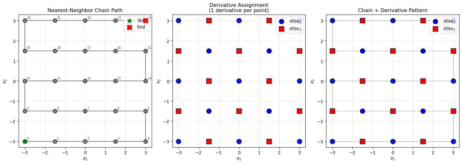
Spatial Chain Construction#
The spatial chain connects training points via a greedy nearest-neighbor traversal. Starting from point 0, we iteratively add the nearest unvisited point to form a connected chain that traverses the space smoothly.
def build_spatial_chain(X_train):
    """
    Build a greedy nearest-neighbor chain through all training points.
    """
    n_pts = len(X_train)
    visited = [False] * n_pts
    chain = [0]
    visited[0] = True

    for _ in range(n_pts - 1):
        current = chain[-1]
        dists = np.linalg.norm(X_train - X_train[current], axis=1)
        dists[visited] = np.inf
        nearest = np.argmin(dists)
        chain.append(nearest)
        visited[nearest] = True

    return chain
Derivative Assignment#
Derivatives are assigned by cycling through dimensions based on chain position. Each point receives exactly one derivative observation.
def assign_cycling_derivatives(chain, n_bases=2):
    """
    Assign derivatives cycling through dimensions along the chain.

    For 2D:
    - position 0, 2, 4, ... -> d/dx1
    - position 1, 3, 5, ... -> d/dx2
    """
    derivative_groups = [[] for _ in range(n_bases)]

    for pos, pt_idx in enumerate(chain):
        group = pos % n_bases
        derivative_groups[group].append(pt_idx)

    return derivative_groups
Training Data Generation#
We generate training points on a regular grid and evaluate the function with derivatives using automatic differentiation.
def generate_grid_points(grid_size, lower_bounds, upper_bounds):
    """Generate training points on a regular grid."""
    x1 = np.linspace(lower_bounds[0], upper_bounds[0], grid_size)
    x2 = np.linspace(lower_bounds[1], upper_bounds[1], grid_size)
    X1_grid, X2_grid = np.meshgrid(x1, x2)
    X_train = np.column_stack([X1_grid.ravel(), X2_grid.ravel()])
    return X_train


def evaluate_function_with_derivatives(X_train, n_bases, n_order):
    """Evaluate function and all first-order derivatives at training points."""
    X_train_pert = oti.array(X_train)
    for i in range(n_bases):
        X_train_pert[:, i] += oti.e(i + 1, order=n_order)

    y_train_hc = true_function(X_train_pert, alg=oti)

    y_values = y_train_hc.real
    all_derivatives = {}
    for i in range(n_bases):
        all_derivatives[i + 1] = y_train_hc.get_deriv([[i + 1, 1]])

    return y_values, all_derivatives
DEGP Setup Functions#
We define two setup functions: one for the cycling strategy (1 derivative per point) and one for the full strategy (all derivatives at all points) as a baseline.
Cycling Strategy#
def setup_cycling_degp(X_train, y_values, all_derivatives, derivative_groups):
    """
    Set up DEGP with cycling derivative assignment.
    Each point contributes exactly one derivative observation.
    """
    # Function values at all points
    y_train_list = [y_values.reshape(-1, 1)]

    # Each derivative only at its assigned points
    for i, group_pts in enumerate(derivative_groups):
        var_idx = i + 1
        y_train_list.append(all_derivatives[var_idx][group_pts].reshape(-1, 1))

    # Derivative indices for first-order derivatives
    der_indices = [
        [[[1, 1]], [[2, 1]]]
    ]

    # Specify which points have which derivatives
    derivative_locations = [list(group) for group in derivative_groups]

    return y_train_list, der_indices, derivative_locations
Full Strategy (Baseline)#
def setup_full_degp(X_train, y_values, all_derivatives):
    """
    Set up DEGP with full derivatives at all points (baseline).
    """
    n_pts = len(X_train)
    all_points = list(range(n_pts))

    y_train_list = [y_values.reshape(-1, 1)]
    for i in range(1, 3):
        y_train_list.append(all_derivatives[i].reshape(-1, 1))

    der_indices = [
        [[[1, 1]], [[2, 1]]]
    ]

    derivative_locations = [all_points, all_points]

    return y_train_list, der_indices, derivative_locations
Model Training#
We initialize the DEGP model and optimize its hyperparameters using PSO
optimization. The model incorporates both function values and selected
derivatives, with derivative_locations specifying where each derivative
is available.
def train_model(X_train, y_train_list, n_order, n_bases, der_indices,
                derivative_locations, normalize_data, kernel, kernel_type):
    """Train DEGP model with PSO optimization."""
    gp_model = degp(
        X_train, y_train_list, n_order, n_bases,
        der_indices,
        derivative_locations=derivative_locations,
        normalize=normalize_data,
        kernel=kernel, kernel_type=kernel_type
    )

    params = gp_model.optimize_hyperparameters(
        optimizer='pso',
        pop_size=200,
        n_generations=30,
        local_opt_every=10,
        debug=True
    )

    return gp_model, params
Interpolation Verification#
We verify that the model correctly interpolates training data, checking both function values and derivative values at their specified locations.
def verify_interpolation(gp_model, params, X_train, y_train_list,
                         derivative_locations, model_name="Model"):
    """Verify that the model correctly interpolates training data."""
    print(f"\nInterpolation Verification for {model_name}")
    print("-" * 50)

    y_pred, _ = gp_model.predict(X_train, params, calc_cov=True, return_deriv=True)

    all_passed = True

    # Check function values
    y_func_true = y_train_list[0].flatten()
    y_func_pred = y_pred[0, :].flatten()
    func_error = np.abs(y_func_pred - y_func_true)
    func_max_err = np.max(func_error)
    func_pass = func_max_err < 1e-4
    all_passed = all_passed and func_pass

    status = "✓" if func_pass else "✗"
    print(f"{status} Function values:  max_err = {func_max_err:.2e}")

    # Check derivatives
    derivative_names = ["∂f/∂x₁", "∂f/∂x₂"]

    for i, (deriv_locs, name) in enumerate(zip(derivative_locations, derivative_names)):
        y_deriv_true = y_train_list[i + 1].flatten()
        y_deriv_pred = y_pred[i + 1, :].flatten()[deriv_locs]

        deriv_error = np.abs(y_deriv_pred - y_deriv_true)
        deriv_max_err = np.max(deriv_error)
        deriv_pass = deriv_max_err < 1e-4
        all_passed = all_passed and deriv_pass

        status = "✓" if deriv_pass else "✗"
        print(f"{status} {name} (n={len(deriv_locs):2d}): max_err = {deriv_max_err:.2e}")

    print("-" * 50)
    print(f"{'✓ ALL PASSED' if all_passed else '✗ SOME FAILED'}")

    return all_passed
Evaluation#
We evaluate the model on a fine grid to assess prediction quality.
def evaluate_on_grid(gp_model, params, lower_bounds, upper_bounds, resolution):
    """Evaluate model on a fine grid."""
    x1 = np.linspace(lower_bounds[0], upper_bounds[0], resolution)
    x2 = np.linspace(lower_bounds[1], upper_bounds[1], resolution)
    X1_grid, X2_grid = np.meshgrid(x1, x2)
    X_test = np.column_stack([X1_grid.ravel(), X2_grid.ravel()])

    y_pred, y_var = gp_model.predict(X_test, params, calc_cov=True)
    y_true = true_function(X_test, alg=np)

    return {
        "X1_grid": X1_grid,
        "X2_grid": X2_grid,
        "y_true": y_true.reshape(X1_grid.shape),
        "y_pred": y_pred.reshape(X1_grid.shape),
        "y_var": y_var.reshape(X1_grid.shape),
        "nrmse": utils.nrmse(y_true, y_pred)
    }
Visualization#
We create visualizations to understand the derivative assignment pattern and compare model performance.
Derivative Assignment Visualization#
def visualize_derivative_assignment(X_train, chain, derivative_groups):
    """Visualize the chain and derivative assignments on the 2D grid."""
    fig, axes = plt.subplots(1, 3, figsize=(15, 5))

    colors = ['blue', 'red']
    markers = ['o', 's']
    labels = [r'$\partial f/\partial x_1$', r'$\partial f/\partial x_2$']

    # Panel 1: Chain path
    ax = axes[0]
    chain_coords = X_train[chain]
    ax.plot(chain_coords[:, 0], chain_coords[:, 1], 'k-', alpha=0.5, linewidth=1.5)
    ax.scatter(X_train[:, 0], X_train[:, 1], c='gray', s=80, edgecolor='k', zorder=5)
    ax.scatter(*X_train[chain[0]], c='green', s=150, marker='*', zorder=10, label='Start')
    ax.scatter(*X_train[chain[-1]], c='red', s=150, marker='X', zorder=10, label='End')
    for i, idx in enumerate(chain):
        ax.annotate(str(i), X_train[idx] + np.array([0.1, 0.1]), fontsize=7, alpha=0.7)
    ax.set_xlabel('$x_1$')
    ax.set_ylabel('$x_2$')
    ax.set_title('Nearest-Neighbor Chain Path')
    ax.legend(loc='upper right')
    ax.set_aspect('equal')
    ax.grid(True, alpha=0.3)

    # Panel 2: Derivative assignments
    ax = axes[1]
    for group, color, marker, label in zip(derivative_groups, colors, markers, labels):
        ax.scatter(X_train[group, 0], X_train[group, 1],
                   c=color, s=120, edgecolor='k', marker=marker, label=label)
    ax.set_xlabel('$x_1$')
    ax.set_ylabel('$x_2$')
    ax.set_title('Derivative Assignment\n(1 derivative per point)')
    ax.legend(loc='upper right')
    ax.set_aspect('equal')
    ax.grid(True, alpha=0.3)

    # Panel 3: Combined view
    ax = axes[2]
    chain_coords = X_train[chain]
    ax.plot(chain_coords[:, 0], chain_coords[:, 1], 'k-', alpha=0.3, linewidth=1)
    for group, color, marker, label in zip(derivative_groups, colors, markers, labels):
        ax.scatter(X_train[group, 0], X_train[group, 1],
                   c=color, s=120, edgecolor='k', marker=marker, label=label)
    ax.set_xlabel('$x_1$')
    ax.set_ylabel('$x_2$')
    ax.set_title('Chain + Derivative Pattern')
    ax.legend(loc='upper right')
    ax.set_aspect('equal')
    ax.grid(True, alpha=0.3)

    plt.tight_layout()
    plt.show()
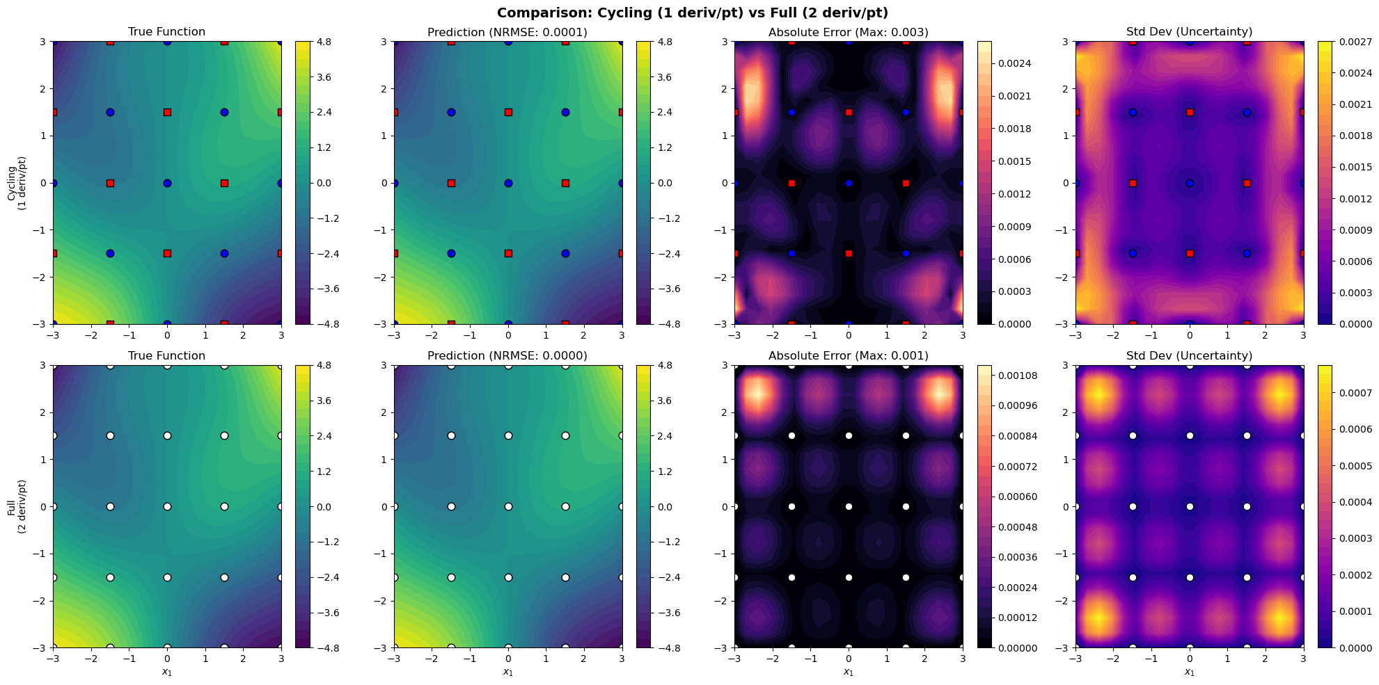
Results Comparison Visualization#
def plot_results_comparison(X_train, results_cycling, results_full, derivative_groups):
    """Compare cycling vs full derivative strategies."""
    fig, axes = plt.subplots(2, 4, figsize=(20, 10))

    colors = ['blue', 'red']
    markers = ['o', 's']

    # Row 1: Cycling strategy
    im0 = axes[0, 0].contourf(results_cycling["X1_grid"], results_cycling["X2_grid"],
                               results_cycling["y_true"], levels=30, cmap="viridis")
    for i, (group, color, marker) in enumerate(zip(derivative_groups, colors, markers)):
        axes[0, 0].scatter(X_train[group, 0], X_train[group, 1],
                           c=color, s=60, edgecolor='k', marker=marker)
    axes[0, 0].set_title("True Function")
    axes[0, 0].set_ylabel("Cycling\n(1 deriv/pt)")
    plt.colorbar(im0, ax=axes[0, 0])

    im1 = axes[0, 1].contourf(results_cycling["X1_grid"], results_cycling["X2_grid"],
                               results_cycling["y_pred"], levels=30, cmap="viridis")
    for i, (group, color, marker) in enumerate(zip(derivative_groups, colors, markers)):
        axes[0, 1].scatter(X_train[group, 0], X_train[group, 1],
                           c=color, s=60, edgecolor='k', marker=marker)
    axes[0, 1].set_title(f"Prediction (NRMSE: {results_cycling['nrmse']:.4f})")
    plt.colorbar(im1, ax=axes[0, 1])

    error_cycling = np.abs(results_cycling["y_true"] - results_cycling["y_pred"])
    im2 = axes[0, 2].contourf(results_cycling["X1_grid"], results_cycling["X2_grid"],
                               error_cycling, levels=30, cmap="magma")
    for i, (group, color, marker) in enumerate(zip(derivative_groups, colors, markers)):
        axes[0, 2].scatter(X_train[group, 0], X_train[group, 1],
                           c=color, s=60, edgecolor='k', marker=marker)
    axes[0, 2].set_title(f"Absolute Error (Max: {error_cycling.max():.3f})")
    plt.colorbar(im2, ax=axes[0, 2])

    im3 = axes[0, 3].contourf(results_cycling["X1_grid"], results_cycling["X2_grid"],
                               np.sqrt(results_cycling["y_var"]), levels=30, cmap="plasma")
    for i, (group, color, marker) in enumerate(zip(derivative_groups, colors, markers)):
        axes[0, 3].scatter(X_train[group, 0], X_train[group, 1],
                           c=color, s=60, edgecolor='k', marker=marker)
    axes[0, 3].set_title("Std Dev (Uncertainty)")
    plt.colorbar(im3, ax=axes[0, 3])

    # Row 2: Full derivatives
    im4 = axes[1, 0].contourf(results_full["X1_grid"], results_full["X2_grid"],
                               results_full["y_true"], levels=30, cmap="viridis")
    axes[1, 0].scatter(X_train[:, 0], X_train[:, 1], c='white', s=60, edgecolor='k')
    axes[1, 0].set_title("True Function")
    axes[1, 0].set_ylabel("Full\n(2 deriv/pt)")
    axes[1, 0].set_xlabel("$x_1$")
    plt.colorbar(im4, ax=axes[1, 0])

    im5 = axes[1, 1].contourf(results_full["X1_grid"], results_full["X2_grid"],
                               results_full["y_pred"], levels=30, cmap="viridis")
    axes[1, 1].scatter(X_train[:, 0], X_train[:, 1], c='white', s=60, edgecolor='k')
    axes[1, 1].set_title(f"Prediction (NRMSE: {results_full['nrmse']:.4f})")
    axes[1, 1].set_xlabel("$x_1$")
    plt.colorbar(im5, ax=axes[1, 1])

    error_full = np.abs(results_full["y_true"] - results_full["y_pred"])
    im6 = axes[1, 2].contourf(results_full["X1_grid"], results_full["X2_grid"],
                               error_full, levels=30, cmap="magma")
    axes[1, 2].scatter(X_train[:, 0], X_train[:, 1], c='white', s=60, edgecolor='k')
    axes[1, 2].set_title(f"Absolute Error (Max: {error_full.max():.3f})")
    axes[1, 2].set_xlabel("$x_1$")
    plt.colorbar(im6, ax=axes[1, 2])

    im7 = axes[1, 3].contourf(results_full["X1_grid"], results_full["X2_grid"],
                               np.sqrt(results_full["y_var"]), levels=30, cmap="plasma")
    axes[1, 3].scatter(X_train[:, 0], X_train[:, 1], c='white', s=60, edgecolor='k')
    axes[1, 3].set_title("Std Dev (Uncertainty)")
    axes[1, 3].set_xlabel("$x_1$")
    plt.colorbar(im7, ax=axes[1, 3])

    plt.suptitle("Comparison: Cycling (1 deriv/pt) vs Full (2 deriv/pt)",
                 fontsize=14, fontweight='bold')
    plt.tight_layout()
    plt.show()
Full Workflow#
Finally, we run the full workflow: generate training data, build the spatial chain, assign cycling derivatives, train both models, and compare results.
# Generate training points on grid
X_train = generate_grid_points(grid_size, lower_bounds, upper_bounds)
print(f"Grid: {grid_size}x{grid_size} = {len(X_train)} points")

# Evaluate function and derivatives
y_values, all_derivatives = evaluate_function_with_derivatives(X_train, n_bases, n_order)

# Build spatial chain and assign derivatives
chain = build_spatial_chain(X_train)
derivative_groups = assign_cycling_derivatives(chain, n_bases)
print(f"d/dx1 assigned to: {len(derivative_groups[0])} points")
print(f"d/dx2 assigned to: {len(derivative_groups[1])} points")

# Visualize the chain and derivative assignments
visualize_derivative_assignment(X_train, chain, derivative_groups)
Grid: 5x5 = 25 points
d/dx1 assigned to: 13 points
d/dx2 assigned to: 12 points
# Setup and train cycling model
print("Training CYCLING derivative model...")
y_train_cyc, der_indices_cyc, der_locs_cyc = setup_cycling_degp(
    X_train, y_values, all_derivatives, derivative_groups
)

total_obs_cyc = sum(y.shape[0] for y in y_train_cyc)
print(f"Total observations: {total_obs_cyc}")

gp_model_cyc, params_cyc = train_model(
    X_train, y_train_cyc, n_order, n_bases, der_indices_cyc, der_locs_cyc,
    normalize_data, kernel, kernel_type
)

verify_interpolation(gp_model_cyc, params_cyc, X_train, y_train_cyc,
                     der_locs_cyc, model_name="Cycling DEGP")
Training CYCLING derivative model...
Total observations: 50
New best for swarm at iteration 1: [ 0.02288031 -0.0687752   0.21318409 -4.11411214] -19.2208479150975
Best after iteration 1: [ 0.02288031 -0.0687752   0.21318409 -4.11411214] -19.2208479150975
Best after iteration 2: [ 0.02288031 -0.0687752   0.21318409 -4.11411214] -19.2208479150975
Best after iteration 3: [ 0.02288031 -0.0687752   0.21318409 -4.11411214] -19.2208479150975
Best after iteration 4: [ 0.02288031 -0.0687752   0.21318409 -4.11411214] -19.2208479150975
New best for swarm at iteration 5: [-0.0508107  -0.06230424  0.23172383 -5.94766267] -27.40363861455736
Best after iteration 5: [-0.0508107  -0.06230424  0.23172383 -5.94766267] -27.40363861455736
New best for swarm at iteration 6: [-0.12007599 -0.13490332  0.52319077 -3.94685222] -28.826155060512313
New best for swarm at iteration 6: [-0.04749708 -0.13959783  0.36342653 -5.72139088] -29.49213867317959
Best after iteration 6: [-0.04749708 -0.13959783  0.36342653 -5.72139088] -29.49213867317959
Best after iteration 7: [-0.04749708 -0.13959783  0.36342653 -5.72139088] -29.49213867317959
New best for swarm at iteration 8: [-0.11477947 -0.0852649   0.4309043  -5.7639108 ] -29.84201226299073
New best for swarm at iteration 8: [-0.10605811 -0.11692424  0.4164234  -6.04956514] -30.186114556422844
Best after iteration 8: [-0.10605811 -0.11692424  0.4164234  -6.04956514] -30.186114556422844
New best for swarm at iteration 9: [-0.08714331 -0.14513165  0.46615839 -5.75502978] -30.22703927158306
New best for swarm at iteration 9: [-0.09074826 -0.1297958   0.42268464 -6.57984822] -30.719035474042478
Best after iteration 9: [-0.09074826 -0.1297958   0.42268464 -6.57984822] -30.719035474042478
New best for swarm at iteration 10: [-0.09275524 -0.11647932  0.42083124 -4.92726718] -30.95667952742479
Gradient refinement improved
Best after iteration 10: [-0.08535655 -0.11865178  0.40388759 -4.92727385] -31.016018593263787
Best after iteration 11: [-0.08535655 -0.11865178  0.40388759 -4.92727385] -31.016018593263787
Best after iteration 12: [-0.08535655 -0.11865178  0.40388759 -4.92727385] -31.016018593263787
Best after iteration 13: [-0.08535655 -0.11865178  0.40388759 -4.92727385] -31.016018593263787
Best after iteration 14: [-0.08535655 -0.11865178  0.40388759 -4.92727385] -31.016018593263787
Best after iteration 15: [-0.08535655 -0.11865178  0.40388759 -4.92727385] -31.016018593263787
Best after iteration 16: [-0.08535655 -0.11865178  0.40388759 -4.92727385] -31.016018593263787
Best after iteration 17: [-0.08535655 -0.11865178  0.40388759 -4.92727385] -31.016018593263787
Best after iteration 18: [-0.08535655 -0.11865178  0.40388759 -4.92727385] -31.016018593263787
Best after iteration 19: [-0.08535655 -0.11865178  0.40388759 -4.92727385] -31.016018593263787
Gradient refinement improved
Best after iteration 20: [-0.0853565  -0.11865223  0.40388793 -4.92727433] -31.016018593634037
Best after iteration 21: [-0.0853565  -0.11865223  0.40388793 -4.92727433] -31.016018593634037
Best after iteration 22: [-0.0853565  -0.11865223  0.40388793 -4.92727433] -31.016018593634037
Best after iteration 23: [-0.0853565  -0.11865223  0.40388793 -4.92727433] -31.016018593634037
New best for swarm at iteration 24: [-0.08539533 -0.11867221  0.40415898 -4.98375729] -31.016032165225248
Best after iteration 24: [-0.08539533 -0.11867221  0.40415898 -4.98375729] -31.016032165225248
Best after iteration 25: [-0.08539533 -0.11867221  0.40415898 -4.98375729] -31.016032165225248
Best after iteration 26: [-0.08539533 -0.11867221  0.40415898 -4.98375729] -31.016032165225248
New best for swarm at iteration 27: [-0.08530748 -0.11866624  0.40380725 -4.97325889] -31.016033455735176
New best for swarm at iteration 27: [-0.08538567 -0.11861152  0.40398388 -5.03963891] -31.016049598485885
Best after iteration 27: [-0.08538567 -0.11861152  0.40398388 -5.03963891] -31.016049598485885
Best after iteration 28: [-0.08538567 -0.11861152  0.40398388 -5.03963891] -31.016049598485885
New best for swarm at iteration 29: [-0.08538199 -0.11864571  0.40401986 -5.03429086] -31.01605112072047
Best after iteration 29: [-0.08538199 -0.11864571  0.40401986 -5.03429086] -31.01605112072047
New best for swarm at iteration 30: [-0.08539519 -0.11861289  0.4040253  -5.05241157] -31.016051149073512
Stopping: Objective improvement < 1e-06

Interpolation Verification for Cycling DEGP
--------------------------------------------------
Note: derivs_to_predict is None. Predictions will include all derivatives used in training: [[[1, 1]], [[2, 1]]]
✓ Function values:  max_err = 4.81e-08
✓ ∂f/∂x₁ (n=13): max_err = 1.28e-08
✓ ∂f/∂x₂ (n=12): max_err = 1.21e-08
--------------------------------------------------
✓ ALL PASSED
True
# Setup and train full model
print("Training FULL derivative model...")
y_train_full, der_indices_full, der_locs_full = setup_full_degp(
    X_train, y_values, all_derivatives
)

total_obs_full = sum(y.shape[0] for y in y_train_full)
print(f"Total observations: {total_obs_full}")

gp_model_full, params_full = train_model(
    X_train, y_train_full, n_order, n_bases, der_indices_full, der_locs_full,
    normalize_data, kernel, kernel_type
)

verify_interpolation(gp_model_full, params_full, X_train, y_train_full,
                     der_locs_full, model_name="Full DEGP")
Training FULL derivative model...
Total observations: 75
New best for swarm at iteration 1: [ 0.02288031 -0.0687752   0.21318409 -4.11411214] -123.33388920288938
New best for swarm at iteration 1: [ -0.19066433   0.01431146   0.69548005 -13.82417601] -127.32397152610214
Best after iteration 1: [ -0.19066433   0.01431146   0.69548005 -13.82417601] -127.32397152610214
Best after iteration 2: [ -0.19066433   0.01431146   0.69548005 -13.82417601] -127.32397152610214
New best for swarm at iteration 3: [ -0.12690935  -0.11434224   0.75382203 -13.74870947] -146.44656549544442
Best after iteration 3: [ -0.12690935  -0.11434224   0.75382203 -13.74870947] -146.44656549544442
New best for swarm at iteration 4: [ -0.09769236  -0.03711586   0.30324901 -13.44328683] -147.25263344398905
Best after iteration 4: [ -0.09769236 -0.03711586 0.30324901 -13.44328683] -147.25263344398905
New best for swarm at iteration 5: [ -0.15501146  -0.13573274   0.85648248 -14.6955153 ] -152.3960574265693
New best for swarm at iteration 5: [ -0.13395107  -0.08959333   0.41961897 -14.27738139] -162.84981979495956
Best after iteration 5: [ -0.13395107  -0.08959333   0.41961897 -14.27738139] -162.84981979495956
Best after iteration 6: [ -0.13395107  -0.08959333   0.41961897 -14.27738139] -162.84981979495956
Best after iteration 7: [ -0.13395107  -0.08959333   0.41961897 -14.27738139] -162.84981979495956
New best for swarm at iteration 8: [ -0.16247549  -0.07478262   0.53312337 -14.10711649] -163.01974287924992
New best for swarm at iteration 8: [ -0.15821438  -0.09353034   0.50117283 -14.1276283 ] -164.57903802021508
Best after iteration 8: [ -0.15821438  -0.09353034   0.50117283 -14.1276283 ] -164.57903802021508
New best for swarm at iteration 9: [ -0.14626119  -0.0929051    0.50248213 -14.43815329] -164.60132747380902
New best for swarm at iteration 9: [ -0.15337719  -0.09807297   0.56059519 -14.02464198] -164.8403228481539
New best for swarm at iteration 9: [ -0.16188463  -0.10545082   0.56032827 -13.58037966] -165.08063077907536
Best after iteration 9: [ -0.16188463  -0.10545082   0.56032827 -13.58037966] -165.08063077907536
New best for swarm at iteration 10: [ -0.14811099  -0.11499776   0.5471476  -14.20583125] -165.1692048973499
New best for swarm at iteration 10: [ -0.15101411  -0.1002371    0.52931802 -14.40200458] -165.22345402620596
Best after iteration 10: [ -0.15101411  -0.1002371    0.52931802 -14.40200458] -165.22345402620596
Best after iteration 11: [ -0.15101411  -0.1002371    0.52931802 -14.40200458] -165.22345402620596
Best after iteration 12: [ -0.15101411  -0.1002371    0.52931802 -14.40200458] -165.22345402620596
New best for swarm at iteration 13: [ -0.15461718  -0.10571339   0.54457239 -14.35541202] -165.34378017508095
Best after iteration 13: [ -0.15461718  -0.10571339   0.54457239 -14.35541202] -165.34378017508095
New best for swarm at iteration 14: [ -0.14931611  -0.1073631    0.53977202 -14.35645283] -165.34495310635822
New best for swarm at iteration 14: [ -0.15526018  -0.10657786   0.57193915 -14.59520605] -165.3668189915519
Best after iteration 14: [ -0.15526018  -0.10657786   0.57193915 -14.59520605] -165.3668189915519
New best for swarm at iteration 15: [ -0.15405587  -0.10657946   0.56303237 -14.33824331] -165.4004608075848
Best after iteration 15: [ -0.15405587  -0.10657946   0.56303237 -14.33824331] -165.4004608075848
New best for swarm at iteration 16: [ -0.15450122  -0.10754283   0.56690413 -14.45745509] -165.4086243137519
New best for swarm at iteration 16: [ -0.15306537  -0.10946025   0.56396755 -14.45471107] -165.4200427376618
Best after iteration 16: [ -0.15306537  -0.10946025   0.56396755 -14.45471107] -165.4200427376618
Best after iteration 17: [ -0.15306537  -0.10946025   0.56396755 -14.45471107] -165.4200427376618
Best after iteration 18: [ -0.15306537  -0.10946025   0.56396755 -14.45471107] -165.4200427376618
New best for swarm at iteration 19: [ -0.15357567  -0.10871637   0.56164463 -14.49533062] -165.42127523058616
Best after iteration 19: [ -0.15357567  -0.10871637   0.56164463 -14.49533062] -165.42127523058616
New best for swarm at iteration 20: [ -0.15339026  -0.10885726   0.5628782  -14.41639266] -165.42135058008193
Gradient refinement improved
Best after iteration 20: [ -0.15377983  -0.10883699   0.56366178 -14.41639266] -165.42187181205503
Best after iteration 21: [ -0.15377983  -0.10883699   0.56366178 -14.41639266] -165.42187181205503
Best after iteration 22: [ -0.15377983  -0.10883699   0.56366178 -14.41639266] -165.42187181205503
Best after iteration 23: [ -0.15377983  -0.10883699   0.56366178 -14.41639266] -165.42187181205503
Best after iteration 24: [ -0.15377983  -0.10883699   0.56366178 -14.41639266] -165.42187181205503
Best after iteration 25: [ -0.15377983  -0.10883699   0.56366178 -14.41639266] -165.42187181205503
Best after iteration 26: [ -0.15377983  -0.10883699   0.56366178 -14.41639266] -165.42187181205503
Best after iteration 27: [ -0.15377983  -0.10883699   0.56366178 -14.41639266] -165.42187181205503
Best after iteration 28: [ -0.15377983  -0.10883699   0.56366178 -14.41639266] -165.42187181205503
Best after iteration 29: [ -0.15377983  -0.10883699   0.56366178 -14.41639266] -165.42187181205503
New best for swarm at iteration 30: [ -0.15383823  -0.10878445   0.56359879 -14.41611052] -165.42187325048235
Best after iteration 30: [ -0.15383823  -0.10878445   0.56359879 -14.41611052] -165.42187325048235
Stopping: maximum iterations reached --> 30

Interpolation Verification for Full DEGP
--------------------------------------------------
Note: derivs_to_predict is None. Predictions will include all derivatives used in training: [[[1, 1]], [[2, 1]]]
✓ Function values:  max_err = 1.58e-10
✓ ∂f/∂x₁ (n=25): max_err = 7.98e-11
✓ ∂f/∂x₂ (n=25): max_err = 5.01e-11
--------------------------------------------------
✓ ALL PASSED
True
# Evaluate both models
results_cyc = evaluate_on_grid(gp_model_cyc, params_cyc, lower_bounds,
                                upper_bounds, test_resolution)
results_full = evaluate_on_grid(gp_model_full, params_full, lower_bounds,
                                 upper_bounds, test_resolution)

print(f"Cycling NRMSE:  {results_cyc['nrmse']:.6f}")
print(f"Full NRMSE:     {results_full['nrmse']:.6f}")
print(f"Ratio:          {results_cyc['nrmse']/results_full['nrmse']:.3f}")

# Plot comparison
plot_results_comparison(X_train, results_cyc, results_full, derivative_groups)
Cycling NRMSE:  0.000074
Full NRMSE:     0.000025
Ratio:          2.945
Results Summary#
For a 5×5 grid (25 training points):
Strategy |
Function Values |
Derivative Obs |
Total Observations |
|---|---|---|---|
Cycling |
25 |
25 (1 per pt) |
50 |
Full |
25 |
50 (2 per pt) |
75 |
Observation reduction: 33%
# Print summary
print("=" * 60)
print("SUMMARY")
print("=" * 60)
print(f"Training points:              {len(X_train)}")
print(f"Dimensions:                   {n_bases}")
print()
print("Cycling strategy:")
print(f"  Function values:            {len(X_train)}")
print(f"  Derivative obs (1 per pt):  {len(X_train)}")
print(f"  Total observations:         {total_obs_cyc}")
print()
print("Full derivative strategy:")
print(f"  Function values:            {len(X_train)}")
print(f"  Derivative obs (2 per pt):  {len(X_train) * 2}")
print(f"  Total observations:         {total_obs_full}")
print()
print(f"Observation reduction:        {(1 - total_obs_cyc/total_obs_full)*100:.1f}%")
print(f"NRMSE ratio (cyc/full):       {results_cyc['nrmse']/results_full['nrmse']:.3f}")
print("=" * 60)
============================================================
SUMMARY
============================================================
Training points:              25
Dimensions:                   2

Cycling strategy:
  Function values:            25
  Derivative obs (1 per pt):  25
  Total observations:         50

Full derivative strategy:
  Function values:            25
  Derivative obs (2 per pt):  50
  Total observations:         75

Observation reduction:        33.3%
NRMSE ratio (cyc/full):       2.945
============================================================
Extension to Higher Dimensions#
For a d-dimensional problem, the cycling pattern extends naturally. Each point in the chain receives one derivative, cycling through all dimensions:
def assign_cycling_derivatives(chain, n_bases):
    """Cycle through all d dimensions along the chain."""
    derivative_groups = [[] for _ in range(n_bases)]

    for pos, pt_idx in enumerate(chain):
        group = pos % n_bases  # Cycles 0, 1, 2, ..., d-1, 0, 1, ...
        derivative_groups[group].append(pt_idx)

    return derivative_groups
For 4D, the pattern becomes:
Position 0, 4, 8, … → ∂f/∂x₁
Position 1, 5, 9, … → ∂f/∂x₂
Position 2, 6, 10, … → ∂f/∂x₃
Position 3, 7, 11, … → ∂f/∂x₄
This achieves a 75% reduction in derivative observations for 4D problems.
Key Takeaways#
Spatial correlation enables information sharing: The GP correlation structure allows derivative information to propagate between neighboring points.
Strategic placement matters: By cycling derivatives along a spatial chain, neighboring points have complementary information.
Trade-off: The cycling strategy reduces computational cost at the potential expense of some accuracy. The effectiveness depends on:
The length scale of the GP relative to point spacing
The smoothness of the underlying function
The spatial distribution of training points